Convexification is often described as a solver strategy, but in trajectory optimization it can make three mathematically different promises. A relaxation may reveal that a structured nonconvex problem was convex in disguise. A sequence of local models may recover useful convexity after nonlinear dynamics destroy that structure. Or the continuous problem may be reformulated so that a finite transcription records information that isolated nodes omit. These promises answer different questions: whether one convex solve recovers the original optimum, whether repeated convex solves approach a stationary trajectory, and whether the computed trajectory represents a continuous-time path claim.

Consider a path-constrained optimal-control problem:

Several difficulties are compressed into this notation. The dynamics may be nonlinear, the control set nonconvex, the final time unknown, and state or obstacle constraints curved. Discretization adds a different issue: satisfying a constraint at finitely many nodes is not the same statement as satisfying it at every time.

Convexity is therefore not merely a choice of solver. It describes what remains of the original problem after a change of variables, a relaxation, or a local approximation. In the line of work considered here, that meaning changes three times:

• Lossless convexification (LCvx) exposes a convex formulation hidden inside a specially structured nonconvex problem.

• Successive convexification (SCvx) constructs a new local convex model at every outer iteration when no globally exact one-shot formulation is available.

• Continuous-Time SCvx (CT-SCvx) first changes how path constraints are represented, then applies a prox-linear method to the resulting finite-dimensional problem.

LCvx is the conceptual and historical beginning of this research line, rather than a mathematical prerequisite for SCvx. The common subject is convexification; the object being convexified, and therefore the conclusion one may draw, changes at each stage. The development below follows that change by asking the same four questions each time: what failed, what changed mathematically, what did the change buy, and what limitation remained?

Lossless convexification (LCvx)

Lower thrust-magnitude bound

The landing example in Açıkmeşe and Blackmore’s 2011 paper [1] contains a lower and upper bound on thrust magnitude. Introducing an auxiliary magnitude $\sigma(t)$ gives

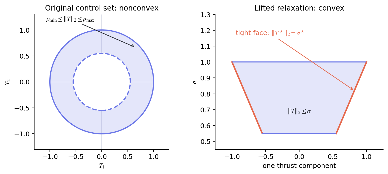
The upper bound describes a Euclidean ball. The positive lower bound removes its center, producing an annulus in two dimensions and a spherical shell in three. Two admissible thrust vectors on opposite sides can have an inadmissible average, so the original set is nonconvex.

The lifted inequalities are convex and second-order-cone representable. They are also a relaxation: they allow $\lVert T\rVert_2<\rho_{\min}$ while $\sigma\ge\rho_{\min}$. Lifting makes the problem easier by adding freedom; it does not, by itself, show that the relaxed optimum solves the original problem.

The essential result is the equality in the last line. Under the controllability, terminal-transversality, and strict state-interiority conditions stated in the paper, the relaxed problem admits an optimal control satisfying the original nonconvex magnitude constraint almost everywhere. The proof uses the Pontryagin Minimum Principle: the costate and switching structure determine the optimal control direction, and a persistent positive gap $\sigma-\lVert T\rVert_2$ conflicts with the necessary optimality conditions under the paper’s nondegeneracy assumptions.

The transferable insight is shorter than the proof:

The computational move is lifting. The mathematical move is proving that the added freedom is not useful at an optimum.

Within that structured model, a globally solved convex problem recovers a global solution of the original nonconvex control problem under the theorem’s assumptions. Here “global” belongs to the specified model and its convex transcription. It says nothing about physical effects omitted from the model, numerical integration error, or finite solver tolerances.

Powered-descent formulation

The 2013 soft-landing paper [2] turns this theorem into a complete formulation. For position $r$, velocity $v$, mass $m$, and commanded thrust $T_c$, define log mass, mass-normalized thrust, and its lifted magnitude by

The first cone is the relaxed thrust-magnitude relation. The second is the thrust-pointing constraint. Boundary conditions prescribe the initial state and desired terminal position and velocity; speed and glide-slope bounds are convex state constraints; maximizing terminal log mass is equivalent to maximizing final mass. For fixed final time, these pieces form an SOCP-compatible point-mass landing problem.

The actual paper writes translation in a planet-fixed rotating frame. Coriolis and centrifugal terms therefore appear in its state matrix, but the dynamics remain affine in state and mass-normalized thrust. Suppressing those terms in the display above exposes the conic structure without changing the convexity argument.

The model also separates the landing objective into two convex problems. Problem 3 first minimizes horizontal terminal miss distance while enforcing touchdown altitude and zero terminal velocity. Problem 4 then minimizes fuel subject to achieving no worse than that optimal miss distance. This lexicographic construction prevents fuel economy from being purchased by accepting an avoidable landing error.

The resulting program is complete in the formulation sense: initial and terminal conditions, mass depletion, velocity, glide slope, thrust magnitude, and pointing all appear in one consistent optimization model. For a prescribed time of flight, the solve is convex. When final time is selected outside that formulation, evaluating a bounded set or one-dimensional family of candidate times still differs fundamentally from iterating local models of the entire trajectory.

Two operations in this formulation should not be conflated. The relaxation of the lower thrust bound is the object of the losslessness theorem. After $z=\log m$, the mass-dependent normalized-thrust bounds still contain exponentials; the 2013 construction replaces them with conservative convex approximations about prescribed mass profiles. The former is proved tight under structural assumptions. The latter is an approximation whose conservatism remains part of the finite model.

This is a formulation breakthrough rather than an iterative nonlinear algorithm. It works because the dynamics, objective, boundary conditions, and control geometry have been selected so that one convex program—or a small outer family when a scalar parameter such as final time is searched—retains the relevant optimum.

That architecture has a boundary. Once attitude kinematics, angular velocity, torque, gimbal geometry, and other nonlinear effects enter the state dynamics, the entire problem no longer shares the same one-shot hidden convexity. The next step is not a stronger claim of losslessness, but a different use of convex structure.

Successive convexification (SCvx)

For general nonlinear dynamics $\dot x=f(x,u)$, SCvx begins with a reference trajectory $(\bar x^j,\bar u^j)$ and a first-order model

The affine model can enter a convex subproblem, but linearization creates two new failure modes. The first is artificial infeasibility: approximate dynamics and hard boundary conditions may be mutually inconsistent even when the nonlinear problem is feasible. Mao, Szmuk, and Açıkmeşe [3] add a heavily penalized virtual control $v$:

Virtual control is a feasibility device rather than a physical actuator. It lets an early convex subproblem be solved from a dynamically inconsistent reference. Its norm must become negligible before the trajectory can be interpreted as a solution of the physical dynamics.

The second failure is an untrustworthy step. Far from the reference, a first-order model may expose false descent directions—artificial unboundedness in the paper—or merely predict an improvement that the nonlinear problem does not realize. The 2016 algorithm bounds the step and asks the nonlinear penalized objective to judge the convex prediction:

A poor ratio rejects the candidate and contracts $\Delta_j$; a good ratio accepts it and may enlarge the next region. The mechanism can be read as a short loop:

reference trajectory
→ local affine model with virtual control
→ convex subproblem inside a trust region
→ nonlinear model-agreement test
→ accept or reject, then update the radius

Repeated convexification is therefore different from repeated relaxation in the LCvx sense. LCvx proves that one enlarged feasible set is tight for a structured problem. SCvx leaves the general problem nonconvex and asks each convex model only for a locally useful step.

The 2016 algorithmic exposition assumes that state and control constraints are already convex or have been convexified separately; nonlinear dynamics are the principal object linearized successively. Its convergence analysis is posed in continuous function spaces, independent of one particular numerical transcription.

A software implementation must nevertheless parameterize controls and discretize or integrate the local dynamics. The accuracy of that finite representation remains a separate question.

This also explains why SCvx can start from a trajectory that does not satisfy the dynamics. Virtual control prevents an early dead end, while the trust mechanism limits the effect of an inaccurate model.

The result remains local: the reference influences the basin reached, and a stationary point of a generic nonlinear OCP need not be globally optimal. The cart-pole experiment later makes this separation visible, first through the failure of one affine model and then through repeated repair of nonlinear dynamic agreement.

An algorithmic skeleton is not yet a flight solver. Time, controls, sensitivities, scaling, and nonlinear validation must all be specified before the loop becomes an implementation.

SCvx for free-final-time 6-DoF powered descent

The 2018 free-final-time Mars landing paper [4] supplies that architecture. Its state contains position, velocity, a scalar-first attitude quaternion, angular velocity, and mass. A gimbaled engine produces force and torque, while final time is itself optimized. The transferable contribution is less the list of rigid-body equations than the route from those equations to a sequence of scaled SOCPs.

The state already shows why the point-mass construction no longer closes in one step. Quaternion kinematics couple attitude and angular velocity; rotational acceleration contains $\omega\times J\omega$; attitude rotates body-frame thrust into the inertial frame; and normalized dynamics couple every state equation to final time.

Upper thrust, gimbal angle, glide slope, and angular-rate bounds retain convex forms. The remaining nonlinear expressions are linearized about the current trajectory, so the solver preserves exact convex pieces and approximates only the obstruction to the next convex subproblem.

Physical time $t\in[0,t_f]$ is mapped to normalized time $\tau\in[0,1]$. The final time becomes a dilation variable coupled to the dynamics. With first-order-hold (FOH) control, continuous-time linearization and interval integration give a discrete local model of the form

The matrices are obtained by more than freezing the dynamics for an Euler step. Along each reference segment, the state-transition matrix is integrated together with sensitivities to the left and right FOH controls and to final time. The resulting map carries the continuous-time linearized model across the interval.

This is the source of the phrase “exact discretization” in the paper. Its scope is narrow: the discrete relation above is the exact interval map of the linear time-varying local model if the associated matrix differential equations are integrated exactly. The nonlinear dynamics have still been linearized, and software evaluates the state and sensitivity equations to finite numerical tolerance.

One outer iteration can be summarized without a separate solver diagram:

reference trajectory
→ propagate the nonlinear reference and integrate sensitivities
→ assemble and scale one SOCP
→ solve for a candidate trajectory
→ update the reference and repeat

Nondimensionalization keeps quaternion components, angular rates, positions, thrust, mass, and time on comparable numerical scales. Virtual control relaxes the discrete dynamics, while a penalized trust term discourages large changes from the reference. This 2018 implementation uses a soft trust treatment and tests virtual control and iterate changes at termination. That is a distinct algorithmic choice from the ratio-managed hard trust region in the 2016 presentation.

Initialization shows how the pieces cooperate. The paper begins from simple state and thrust profiles that need not satisfy the nonlinear rigid-body equations. The first propagation records their local sensitivities, virtual control makes the boundary-value subproblem solvable, and the trust penalty keeps the candidate near information supplied by the reference.

Each accepted trajectory then supplies the next nominal flow and interval matrices. Dynamic consistency is recovered through the repeated linearize–integrate–solve cycle instead of being required at initialization.

The paper thereby turns the abstract SCvx loop into a complete free-final-time 6-DoF solver: initialize a reference, propagate and linearize continuously, integrate interval sensitivities, solve a scaled cone program, update the reference, and check nonlinear dynamic consistency. Its examples demonstrate that architecture for the stated vehicle and numerical setup.

The paper also says that this variant is similar, but not identical, to the 2016 SCvx algorithm and does not inherit that convergence proof directly. Its reported timings characterize those implementations rather than every powered-descent problem.

Convergence results and qualifications

Numerical success and a theorem about the generated sequence answer different questions. The 2018/2019 convergence paper [5] studies a finite-dimensional SCvx formulation after nonlinear equalities and inequalities have been placed in an $\ell_1$ exact-penalty objective. Schematically:

Here $\mathcal Z$ contains the remaining convex constraints. Exact penalization connects first-order properties of the nonsmooth penalized problem to those of the constrained problem at a finite penalty weight. Feasibility, a sufficiently large $\lambda$, and the relevant constraint qualifications are what allow a stationary point or local minimizer to recover the corresponding KKT or local-optimality statement. The penalty alone supplies neither feasibility nor global optimality.

Three levels of convergence must then be separated. Weak convergence concerns stationary accumulation points. Strong convergence means that the whole sequence approaches one limit. A superlinear rate is a still more local statement about how quickly iterates approach that limit.

The original paper claimed all three, using a Kurdyka–Łojasiewicz argument for whole-sequence convergence and structural optimal-control assumptions for the local rate. Its word “global” described the reach of the convergence analysis from arbitrary initialization, not convergence to a global minimizer.

The 2024 Remarks paper [6] identifies where this chain overreached. The exact-penalty theorem cited in the first direction of the original Theorem 3.9 requires a local minimizer, rather than merely a KKT point. Bounded iterates require a compact level-set assumption.

More seriously, Eq. (3.33) does not follow from the lemmas used in the KL proof, so Section 3.2 does not establish strong convergence under its original assumptions. The superlinear proof also needs the entire sequence to converge to the same point; convergence of one subsequence is insufficient.

The note reconnects SCvx to trust-region results of Zhang from 1985 and 1989. With compact level sets, the stationary-accumulation-point result remains the baseline conclusion. Strong convergence and the superlinear rate can be recovered near a feasible limit under tighter local growth conditions inherited from LICQ, strict complementarity, and a sufficient set of binding constraints.

These conditions are appreciably stronger than a generic claim of “SCvx is superlinear.”

The correction changes the proof and the scope of its conclusions, not the iteration or the reported numerical trajectories. The careful statement is therefore: SCvx has stationary accumulation-point guarantees for the penalized finite problem under compactness and regularity assumptions; feasible stationary points can recover first-order conditions of the constrained problem with a sufficiently large penalty; whole-sequence and superlinear conclusions require stronger local hypotheses.

Even perfect convergence of a node-constrained problem leaves another logical gap untouched.

Continuous-time path-constraint representation

Suppose virtual control is negligible, shooting defects are small, and every grid node satisfies a path inequality. The implication

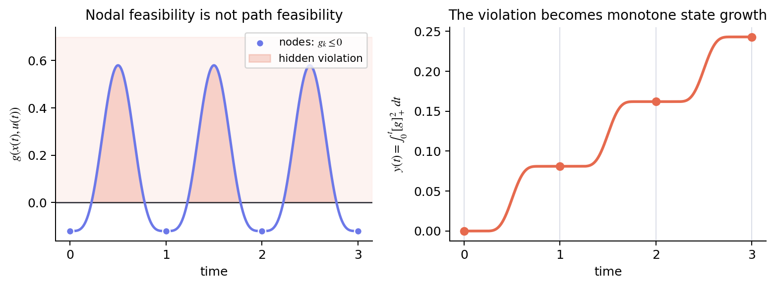
is false. A rocket can cross a glide-slope cone between knots, an interpolated path can enter an obstacle, or a cart can leave its finite track and return before the next node. A finer grid may reduce the observed error, but it still asserts only a larger finite collection of inequalities.

Accumulated violation state

Elango et al. [7] instead put the missing inter-sample information into the dynamics before discretization. For inequalities $g_i(x,u)\le0$ and equalities $h_j(x,u)=0$, one admissible nonnegative exterior measure is

The paper permits a broader class of exterior penalties; the squared positive-part and squared equality residual make the logic immediate. Because $\Lambda\ge0$, $y$ is nondecreasing. Lemma 2 and Corollary 3 show that $y(t_f)=0$ is equivalent to path feasibility almost everywhere along the corresponding trajectory.

If the composed path functions are continuous on an interval, any positive violation persists on a neighborhood and contributes positive area. Zero accumulation then gives pointwise feasibility on that segment.

The change is representational: a path predicate has become an endpoint condition on a monotone state. Multiple shooting will later sample $y$ at interval boundaries, but each increment already contains an integral over the whole interval.

Relaxation of the zero-accumulation condition

Exact zero accumulation creates a constraint-qualification problem. At a feasible point, the gradient of the squared exterior penalty vanishes. Combining the accumulated-state shooting equation with a zero-increment boundary condition then makes active constraint gradients structurally dependent, violating LICQ. The paper uses the positive interval relaxation

The relaxation also has a quantitative interpretation. Under the compact control and dilation sets, bounded path-derivative, and minimum interval-length assumptions of Theorem 14, a scalar path component with derivative bound $\omega$ satisfies

when $\varepsilon\le\omega^2\Delta t_{\min}^3/4$. An analogous absolute-value bound holds for equality constraints. Thus zero accumulation gives the exact almost-everywhere statement, whereas positive $\varepsilon$ gives a conditional violation bound. In computation, the usefulness of that bound depends on defensible derivative constants; dense rollout remains a separate numerical check on the returned trajectory.

Finite-dimensional multiple shooting

The reformulated OCP is made finite-dimensional through control parameterization, generalized time dilation, and multiple shooting. Let $s(\tau)>0$ satisfy $dt/d\tau=s(\tau)$, and collect the physical state, accumulated violation, physical time, and any running-cost state into $\xi$. Over interval $k$,

where $q_k$ contains the interval control and dilation parameters. The nodal values $\xi_k$ are independent shooting variables, and the nonlinear residuals $d_k$ enforce agreement with the interval flow. That flow carries physical dynamics, running cost, elapsed time, and accumulated violation together. Its first derivatives follow from variational differential equations.

Generalized dilation is richer than one scalar final time: the positive function $s(\tau)$ distributes physical duration across intervals. The physical clock satisfies $t’=s$, and the state, running-cost, and violation dynamics receive the same factor. The fixed-final-time notebook experiments do not exercise this layer, but it is part of the general formulation.

As a mathematical object, $\Phi_k$ is the exact solution operator of an initial-value problem. Code approximates it and its sensitivities with a numerical integrator. Reporting both shooting defects and an independently evaluated dense nonlinear rollout keeps that numerical approximation visible.

Convex-composite and prox-linear formulation

After parameterization and multiple shooting, smooth nonlinear flow and boundary residuals are collected in $G(z)$. A convex outer function $H$ contains the terminal cost and $\ell_1$ exact penalties, while $J(z)=\delta_{\mathcal Z}(z)$ retains the directly representable convex constraints. This gives the convex-composite objective and its prox-linear model:

Here $\gamma$ is the exact-penalty weight and $\rho_j$ sets the proximal step scale. Each layer has one role: $G$ preserves nonlinear flow information, $H$ preserves convex nonsmooth structure, $DG(z^j)$ supplies the local model, and the proximal term controls its locality. The last term plays a trust-like role, but the subproblem and analysis now come from convex-composite minimization rather than the hard-radius presentation of 2016.

CT-SCvx is therefore more than SCvx with one extra state. It changes the OCP representation, the finite multiple-shooting problem, and the optimization framework applied to that problem.

Under the paper’s smoothness, boundedness, and proximal-step assumptions, prox-linear iterations approach stationarity of the penalized finite problem. A stationary point that is feasible for the control-parameterized multiple-shooting problem is a KKT point under the stated regularity conditions; conversely, a KKT point is stationary for a sufficiently large finite penalty. For the convex OCP specialization, strong Slater and the penalty/proximal conditions strengthen this correspondence to global minimizers.

The scope remains finite and local: controls are parameterized, flow maps are integrated numerically, $\varepsilon$ and solver tolerances are positive, and the general nonconvex method seeks stationary points. “Continuous-time constraint satisfaction” refers to what the augmented flow represents under the paper’s assumptions. A particular floating-point solution still needs numerical error and residuals to be reported.

Numerical examples

The accompanying executable notebook implements two deliberately reduced tests. It is not the historical code for Refs. 1–7. CVXPY and Clarabel solve the convex subproblems, SciPy integrates flows and variational equations, and a coarse CasADi/IPOPT solve supplies only the cart-pole trajectory family.

The experiments do not force every method onto every model:

3-DoF rocket:
node-only LCvx → continuous-time glide-slope treatment

cart-pole swing-up:
one affine model → node-only SCvx → CT-SCvx

Within each comparison, the grid, control hold, dynamics, scaling, and dense nonlinear evaluator are fixed. The purpose is to separate relaxation tightness, nonlinear dynamic consistency, and inter-sample path behavior.

Rocket: nodal and continuous-time glide-slope constraints

The reduced rocket uses the $K=8$, $t_f=84\,\mathrm{s}$, ZOH setup and physical parameters of the pinned 3-DoF CT-SCvx example. Its state is $[r,v,\log m]$; its control is mass-normalized thrust together with the lifted magnitude. One node-only SOCP, without a nonlinear-programming initializer, supplies the LCvx baseline and the initial reference for the continuous-time glide-slope formulation.

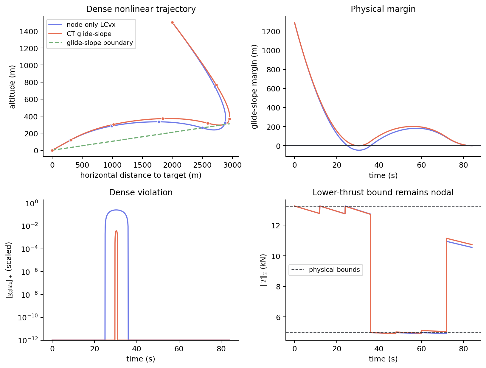
Clarabel reports the LCvx solve as optimal. Its physical lift gap is $3.122\times10^{-3}\,\mathrm N$. The CT solve uses $\varepsilon=10^{-5}$, reaches a maximum $y$ increment of $9.986\times10^{-6}$, and has a scaled shooting defect of $2.204\times10^{-11}$. These are numerical checks on the computed transcription; the small lift gap illustrates the LCvx theorem’s mechanism at the nodes rather than proving the theorem.

The more consequential difference appears between the nodes. The LCvx trajectory penetrates the glide-slope cone by $47.423\,\mathrm m$ under dense rollout. Placing only the glide-slope family in $y$ reduces the same diagnostic to $0.632\,\mathrm m$, with about $1.9\,\mathrm{kg}$ more propellant.

The thrust panel marks the scope of the experiment. The CT trajectory retains a $77.844\,\mathrm N$ inter-sample shortfall in the physical lower-thrust bound because that family remains nodal. The experiment therefore treats glide slope continuously; it does not establish continuous-time feasibility for every rocket constraint.

Cart-pole: dynamic consistency and inter-sample feasibility

Cart-pole enters directly at the SCvx stage: it has smooth nonlinear dynamics, but this experiment has no LCvx-style tight control relaxation. With $x=[p,\theta,\dot p,\dot\theta]^\top$, force $F$, cart mass $M$, pole mass $m$, and pole length $\ell$, the direct input coefficient in angular acceleration is

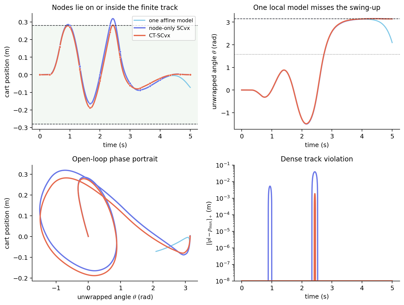
During the swing-up, the dynamics can amplify accumulated integration and transcription errors. This is especially true when the pole moves from angle $\pi/2$ toward $\pi$, and particularly near $\pi/2$, where the cart has poor instantaneous authority over the pole. The light-blue curve in the trajectory figure below shows the one-model open-loop rollout missing the swing-up after this sensitive region. Russ Tedrake’s trajectory-optimization notes and code give a detailed explanation of why trajectory stabilization matters. In this region, even a small mismatch between the simulated state and the nominal trajectory can be amplified significantly, causing the open-loop rollout to miss the swing-up.

This coefficient describes instantaneous input authority, not loss of controllability at $\pi/2$. A dynamically consistent open-loop trajectory also serves a different purpose from feedback stabilization. Integration error, shooting defect, inter-sample constraint violation, and open-loop sensitivity are therefore evaluated as separate properties.

The experiment uses an unwrapped target $\theta(t_f)=\pi$, $t_f=5\,\mathrm{s}$, 16 knots, ZOH force, and the track limit $\lvert p(t)\rvert\le0.28\,\mathrm m$. A deliberately coarse 15-interval nonlinear solve identifies a swing-up family. After resampling and nonlinear rollout, this initializer has a scaled terminal error of $4.682\times10^{-2}$ and reaches $\lvert p\rvert=0.313\,\mathrm m$. Only its primal state and control supply the common reference; no multiplier or barrier state is transferred.

One affine model does not predict the nonlinear open-loop swing-up: the rollout misses the terminal angle by $-1.047\,\mathrm{rad}$, approximately $-\pi/3$. Repeated SCvx reduces the scaled dynamic defect to $4.296\times10^{-10}$ and the virtual-control norm to $1.178\times10^{-13}$; it takes 8 accepted outer steps and 24 convex solves.

The corresponding CT-SCvx values are a $4.155\times10^{-10}$ physical-state defect, a $7.116\times10^{-9}$ augmented-state defect, 53 accepted steps, and 96 convex solves. Its maximum $y$ increment is $9.668\times10^{-7}$ and its normalized accumulated violation is $9.667\times10^{-7}$.

SCvx has repaired local model agreement and dynamic consistency, but its track condition remains nodal. The node-only trajectory satisfies all 16 sampled bounds while leaving the track by $38.7\,\mathrm{mm}$ between them. With the same dynamics, horizon, grid, control hold, initial reference, scaling, objective, and cone solver, CT-SCvx reduces the dense diagnostic to $1.864\,\mathrm{mm}$. Its accumulated violation remains positive, consistent with the relaxed constraint and finite numerical tolerances.

The solve counts provide algorithmic context rather than a speed comparison. The outer methods use different globalization rules, and this implementation is not a matched performance benchmark. A runtime claim would require controlled implementations, repeated measurements, and comparable stopping conditions.

Comparison of LCvx, SCvx, and CT-SCvx

The limits follow the same progression. LCvx applies to a narrow geometry and does not remove transcription error. SCvx has a local solution concept and may enforce path constraints only at nodes. CT-SCvx still uses finite control parameterizations, numerical flow integration, positive tolerances, and local stationarity for nonconvex problems.

The common research style is to expose the convex structure that remains, then make a precise claim about what that structure preserves. At first, convexification acts on the feasible set; then on the local model; finally on the finite representation of a continuous-time claim.

References

1. B. Açıkmeşe and L. Blackmore, “Lossless Convexification of a Class of Optimal Control Problems with Non-Convex Control Constraints”, Automatica, 2011. See Sec. 2, Eqs. (1), (3)–(10), Theorem 2, and the PMP argument in Eqs. (11)–(22).

2. B. Açıkmeşe, J. M. Carson III, and L. Blackmore, “Lossless Convexification of Nonconvex Control Bound and Pointing Constraints of the Soft Landing Optimal Control Problem”, IEEE Transactions on Control Systems Technology, 2013. See Secs. II–IV, Problems 1–4, Theorem 1, and Eqs. (33)–(36).

3. Y. Mao, M. Szmuk, and B. Açıkmeşe, “Successive Convexification of Non-Convex Optimal Control Problems and Its Convergence Properties”, arXiv v3, 2016. See Sec. II, Eqs. (1)–(9), Algorithm 1, and Sec. III.

4. M. Szmuk and B. Açıkmeşe, “Successive Convexification for 6-DoF Mars Rocket Powered Landing with Free-Final-Time”, 2018. See Secs. II–III, Problems 1–2, Eqs. (14)–(27), and Algorithm 1.

5. Y. Mao, M. Szmuk, X. Xu, and B. Açıkmeşe, “Successive Convexification: A Superlinearly Convergent Algorithm for Non-convex Optimal Control Problems”, arXiv v2, 2018/2019. See Secs. 2–4, especially Theorems 3.9, 3.13, and 4.7, together with Ref. 6.

6. Y. Luo, P. Elango, and B. Açıkmeşe, “Remarks on ‘Successive Convexification: A Superlinearly Convergent Algorithm for Non-convex Optimal Control Problems’”, arXiv v2, 2024. See Sec. 2 for the corrections and Sec. 3 for the stronger whole-sequence result.

7. P. Elango et al., “Successive Convexification for Trajectory Optimization with Continuous-Time Constraint Satisfaction”, 2024. See Lemma 2, Corollary 3, Lemma 10, Theorem 14, Algorithm 1, and the stationarity/KKT results in Secs. 4–5.

Reference implementations

• The pinned CT-SCvx implementation directly accompanies Ref. 7.

• SCPToolbox.jl is a later general-purpose reference implementation; its current branch is not the historical code for Refs. 3–4.

• The executable notebook accompanies this article.

ADMM and the proportional–integral projected-gradient family are first-order primal–dual methods for constrained optimization. Both combine a primal update with a constraint-space state driven by residuals, and both rely on simple projections whenever the problem representation permits them. Their principal computational difference lies in the primal update: ADMM evaluates a proximal subproblem—an equality-constrained quadratic program in OSQP—whereas PIPGeq takes an explicit projected-gradient step and returns the constraint correction through $G^\top$. A reusable factorization can make the former inexpensive over a fixed problem family; the latter removes the linear solve from its online iteration, but exposes the iteration more directly to scaling and geometry.

The discussion below begins with the augmented Lagrangian, specializes ADMM to quadratic programs, and then develops the paper lineage $\text{PIPGeq}\rightarrow\text{PIPG}\rightarrow\text{xPIPG}$. This ordering is not a claim that PIPG historically descends from ADMM. It places two related primal–dual constructions on the same problem so that their states, operators, and computational costs can be compared without changing the model.

Dual ascent and the augmented Lagrangian

Consider an equality-constrained convex problem

Its Lagrangian and dual function are

When a minimizer $x^+(y)$ exists and $d$ is differentiable, $\nabla d(y)=Ax^+(y)-b$. Dual ascent therefore alternates between an exact primal minimization and a residual update:

The multiplier already has a concrete dynamical interpretation. For a constant step, it is the initial multiplier plus a running sum of equality residuals. This accumulation is useful, but the unaugmented primal minimization may be nonunique, poorly conditioned, or even unbounded for intermediate multipliers.

The augmented Lagrangian adds a quadratic penalty:

The method of multipliers uses

The penalty regularizes the primal step and makes constraint violation visible inside it. The same term also couples all variables that appear in $Ax-b$. This is the point at which alternating minimization becomes useful.

ADMM

ADMM applies the augmented-Lagrangian idea to a separable problem

With residual $r=Ax+Bz-c$ and scaled multiplier $u=y/\rho$, completing the square gives

One scaled ADMM iteration is then

The first two lines are proximal subproblems evaluated in sequence. The last line integrates the splitting residual:

This is the first structural resemblance to PIPG: both methods carry a constraint-space state with memory. The residuals are nevertheless different. ADMM accumulates the agreement error between split variables, whereas PIPGeq will accumulate the original equality residual $Gz-g$ directly. Their primal maps are also different, so the states should not be identified merely because both are residual sums.

For generic ADMM, the cost of an iteration is the cost of the two proximal operators. They may be scalar formulas, projections, linear solves, or complete inner optimization problems. Statements about ADMM’s linear algebra are therefore meaningful only after a particular splitting has been chosen.

The conventional primal residual is

while the change in the second block produces the familiar dual residual

These are finite-iteration expressions of primal feasibility and stationarity, not merely measures of whether the iterates have stopped moving.

ADMM specialized to a quadratic program

OSQP considers the convex quadratic program

where $P\succeq0$. Introducing $z=Ax$ separates the quadratic objective from the interval $[l,u]$. Projection of $z$ is then a componentwise clip; the other ADMM subproblem is an equality-constrained QP. Writing the possibly diagonal OSQP penalty as $R$, its optimality conditions reduce to

where $R$ is a positive diagonal penalty matrix. The quasi-definite coefficient matrix is independent of the iterates. A direct implementation factors it once and reuses the factors for forward and backward substitution. If $P$, $A$, $\sigma$, or $R$ changes numerically, the numerical factorization changes as well, although an unchanged sparsity pattern can preserve symbolic analysis.

Eliminating $\nu$ gives the positive-definite alternative

This system can also be solved iteratively. That avoids a direct factorization, but it does not remove the linear-system solve; it moves the solve into an inner iteration.

In a dense fixed-matrix implementation, this factor can be reused while $q,l,u$ vary. Each online iteration then applies $A^\top$ and $A$, performs an interval projection, and uses one forward and one backward triangular solve. This is a favorable regime for direct ADMM by construction: the coupled inverse map is paid for once and applied repeatedly through its factors.

For this QP form, it is natural to monitor the KKT residuals directly:

The penalty $R$ is simultaneously an ADMM metric and a form of constraint scaling. A single scalar $\rho$ sets one compromise for every row; a diagonal $R$ can compensate for rows with different units or magnitudes. Adaptive residual balancing changes this metric during the solve, but a direct method must then pay for a new numerical factorization. Preconditioning is already part of the algorithm’s effective geometry, well before PIPG enters the discussion.

PIPGeq

The foundational PIPGeq paper begins from a closely related problem:

with $P\succeq0$, $G\in\mathbb R^{m\times n}$, and a closed convex set $Z$ whose Euclidean projection is inexpensive. In model predictive control, $Gz=g$ typically represents dynamics, while $Z$ is a Cartesian product of state and input sets.

There is one notation change worth making explicit. The 2020 PIPGeq paper calls the objective Hessian $H$ and the equality operator $G$; the later conic papers call the objective Hessian $P$ and the affine operator $H$. I use $P$ for objective curvature throughout, retain $G$ for the equality-only problem, and switch to $H$ only when the general cone is introduced.

Applied to this problem, an ADMM splitting uses two copies of the primal variable: one is constrained by $Gz=g$, and the other by $z\in Z$. The first subproblem in the PIPGeq paper has the KKT system

Here $y$ is the equality-constrained primal copy and $\nu$ is its multiplier. When $P$ and $G$ are fixed, this system is a good candidate for an offline factorization. When they change from one online problem to the next, the same step requires new linear algebra. PIPGeq changes this particular primal update:

The name is literal. With a constant $\beta$,

so $w^k$ is the discrete integral of the equality residual. The term $\beta(Gz^k-g)$ is the instantaneous proportional correction, and $v^k$ is their sum. Finally, $G^\top v^k$ maps this constraint-space signal back to the primal space, where it corrects the objective gradient.

This interpretation is more precise than saying that PIPGeq merely “uses feedback.” Its primal step contains three visible directions:

They are respectively the projected-gradient, proportional, and integral contributions before projection onto $Z$.

The same decomposition can be read directly through the augmented Lagrangian:

The proportional term is therefore not an additional heuristic correction; it is the gradient of the quadratic penalty on the current equality residual. The integral state supplies the multiplier term. This does not turn PIPGeq into ADMM: ADMM minimizes augmented proximal subproblems for a chosen splitting, whereas PIPGeq evaluates this gradient once and projects. It does identify the computational fork precisely. One method applies a coupled inverse map; the other replaces that map by a scalar-step forward approximation.

For the constant-step theorem in the original paper, if $P\preceq\lambda I$ and $G^\top G\preceq\sigma I$, the steps satisfy

The experiment below uses

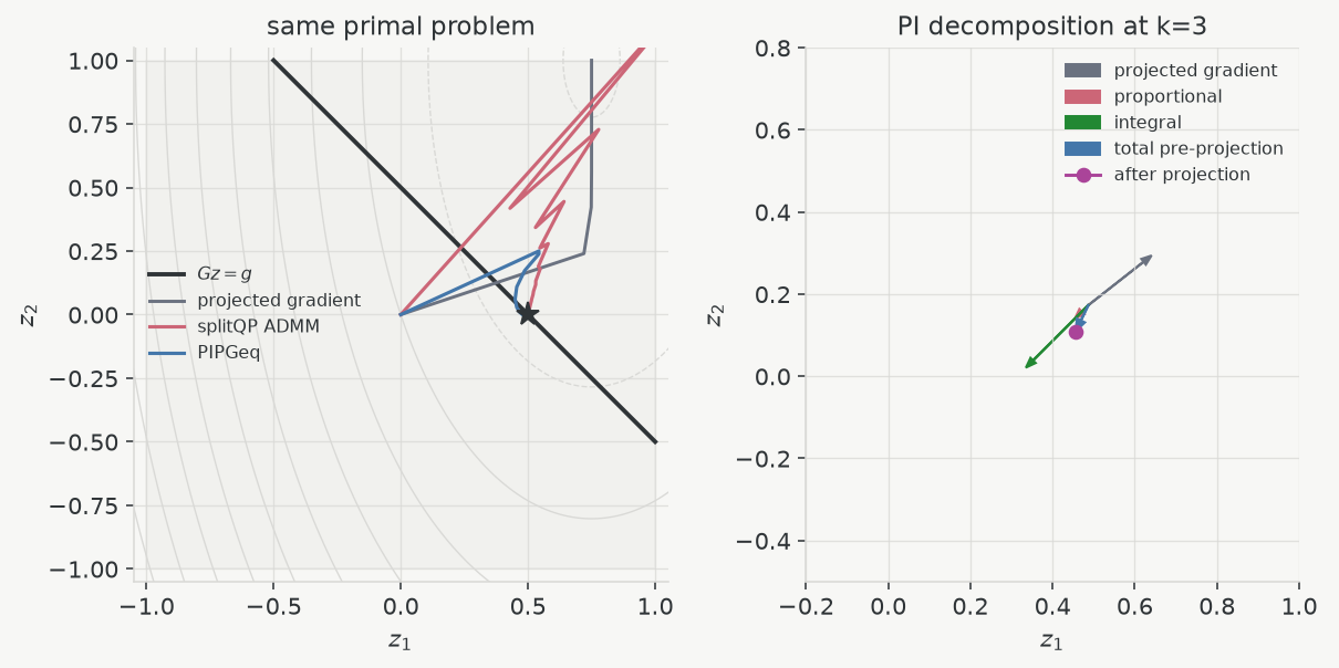
The solution is $z^\star=(0.5,0)$ with $f^\star=-1$. Projected gradient sees the box but not the affine line and therefore converges to the optimum of the wrong problem. ADMM and PIPGeq approach the same constrained solution using different primal maps. The second panel evaluates all three PIPGeq directions at one common iterate; their sum is the trial step before box projection.

On this example, $\lambda=4$, $\sigma=\lVert G\rVert^2=2$, $\beta=\sqrt2$, and $\alpha\approx0.146447$. PIPGeq reaches an equality residual below $10^{-6}$ in about 25 iterations; the factor-reusing ADMM baseline terminates after 104 iterations at its stricter $10^{-9}$ absolute and relative tolerances. These counts describe the chosen parameters and stopping rules, not an intrinsic ordering of the methods.

The online PIPGeq formula contains products with $P$, $G$, and $G^\top$, plus one projection onto $Z$. It contains no linear-system solve. This qualification matters: norm estimation, preconditioning, and code generation are setup work, and $\Pi_{Z}$ may itself be an optimization problem unless $Z$ has a simple product structure. PIPGeq is inexpensive only when these operators are inexpensive.

General conic PIPG

PIPGeq treats $Gz-g=0$. General PIPG considers

where $D\subseteq\mathbb R^n$ is closed and convex and $K\subseteq\mathbb R^m$ is a closed convex cone. The paper uses the polar cone

This sign convention is not cosmetic. If $K^{\ast}={w:\langle w,y\rangle\ge0}$ denotes the usual dual cone, then $K^\circ=-K^{\ast}$. Thus

The saddle representation is

Consequently, the constraint correction must remain in $K^\circ$. PIPG does this with

The first line adds the current conic residual and projects the correction onto the admissible multiplier cone. The second returns that correction through $H^\top$. The final line predicts the correction associated with the new primal point. The pair of dual-side updates is therefore a projected prediction–correction form of the PI state.

For $K=\mathbb R_{+}^{m}$, a negative component of $Hz-g$ is a violation and drives the corresponding correction into the negative orthant; positive feasible slack moves it back toward zero. The polar projection prevents a multiplier with the wrong sign. For an SOC, the same selection is geometric rather than componentwise.

If $K={0}$, the polar projection is the identity. Combining the first and third lines gives

which recovers the equality integral update. For product cones, all projections separate blockwise. Moreau’s decomposition is particularly convenient:

Orthants and second-order cones therefore retain closed-form projections. An arbitrary intersection or rotated polytope need not.

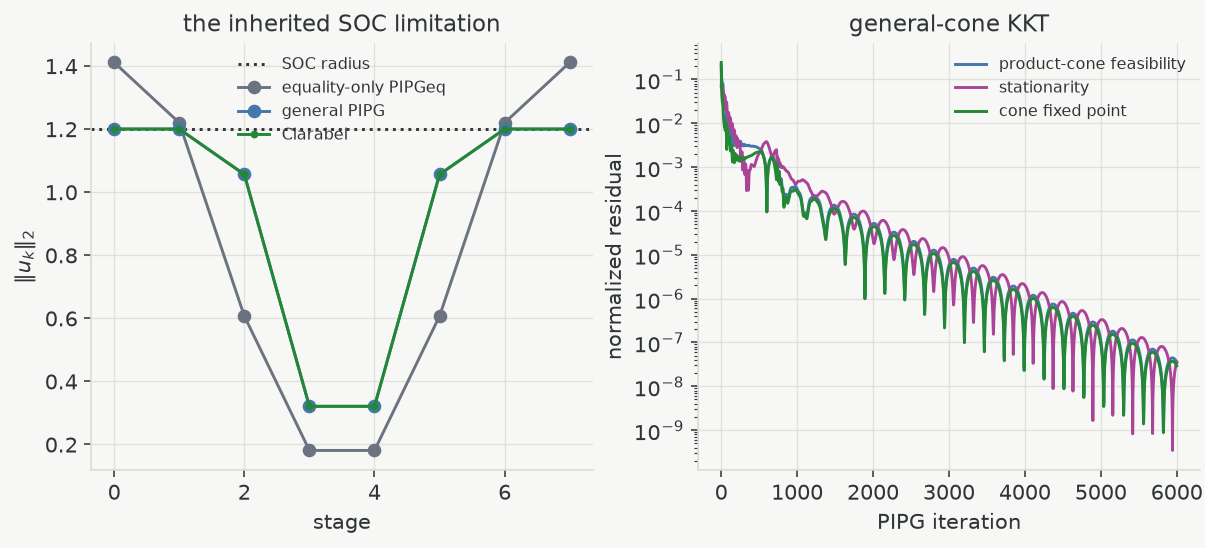
The trajectory experiment below adds a genuine second-order-cone bound on the control norm while keeping the affine dynamics and box bounds unchanged. Equality-only PIPGeq satisfies the dynamics but violates the SOC radius at the outer stages. General PIPG agrees with the independent conic reference and drives feasibility, stationarity, and the cone fixed-point residual down together.

Constant-step PIPG and PDHG

General PIPG is closely related to a constant-step forward variant of PDHG. For constant $\beta$, the final PIPG line from the preceding iteration gives

Substitution into the next polar projection yields

Together with the projected primal-forward step, and after an index shift, this is the constant-step PDHG form displayed in the PIPG paper. The statement is exact but narrow: it does not identify every method called PDHG with PIPG, and it does not make varying-step PIPG or relaxed xPIPG the same iteration.

ADMM is likewise related to Douglas–Rachford splitting, but through a different monotone inclusion and different resolvents. These methods share primal–dual state, projections, residuals, and fixed-point language; they should still be distinguished by the operator evaluated at each iteration.

xPIPG

For the quadratic cone problem

xPIPG writes the iteration in terms of relaxed primal and dual states $(\xi^j,\eta^j)$:

Here $z^{j+1}$ and $w^{j+1}$ are projected base points; $\xi^{j+1}$ and $\eta^{j+1}$ are the fixed-point states carried to the next iteration. With $\rho=1$, the base points become the next states and the unrelaxed PIPG/PDHG representation is recovered. Values $1<\rho<2$ extrapolate the fixed-point map. The argument $2z^{j+1}-\xi^j$ is the reflection of the incoming primal state through its projected point, so the dual projection sees the newest primal correction. This reflected coupling and the relaxation by $\rho$ are fixed-point operations, not Nesterov momentum.

The basic sufficient condition is

Writing $\beta=\omega\alpha$ gives the equivalent upper bound

The open inequalities are important. An implementation normally estimates $\lVert H\rVert$ and keeps a numerical safety margin; the power iteration used for this estimate belongs to setup, not to the recurring xPIPG kernel.

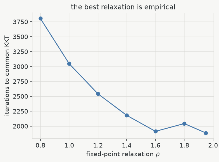
Relaxation changes the transient without changing the underlying fixed points. There is no universal best $\rho$. On the trajectory problem, the same $\alpha$ and $\beta$ were used for $\rho\in{0.8,1.0,1.2,1.4,1.6,1.8,1.95}$. The measured iteration counts to a common KKT target were respectively $3804,3046,2541,2180,1912,2042,$ and $1885$. The best value on this finite grid was $1.95$; the nonmonotone change between $1.6$ and $1.8$ is enough to rule out treating a value reported by one implementation as a universal constant.

Iterate differences and infeasibility

If the conic problem has a primal–dual solution, the xPIPG fixed-point state can converge and consecutive base-point differences approach zero. When no fixed point exists, averaged-operator theory allows the differences to approach a nonzero minimal-displacement direction instead. For diagnostics, it is convenient to remove the primal, dual, and relaxation scales:

Positive rescaling does not change cone membership or the sign of a separation test. The magnitudes $d_{z}^k$ and $d_{w}^k$ are nevertheless only a first indication. A limiting dual direction $\bar w$ certifies primal infeasibility only if it belongs to $K^\circ$ and strictly separates the attainable residuals from $K$:

For a box $D$, the infimum is evaluated exactly by choosing a lower or upper bound according to the sign of each component of $H^\top\bar w$. For a general set, validating the certificate requires a support-function or linear- minimization oracle, which may itself be nontrivial.

A candidate primal direction $\bar z$ certifies dual infeasibility or unboundedness only after the corresponding recession and improvement tests:

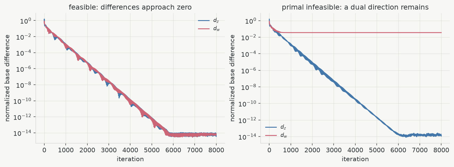
The matched experiment keeps the same dimensions, cone blocks, objective, and steps. Only the conic radius changes. In the feasible instance both normalized differences fall to about $10^{-14}$ and the final KKT residual is $7.9\times10^{-16}$. In the primal-infeasible instance the primal difference vanishes while the dual difference remains near $3.56\times10^{-2}$. The normalized direction has polar-cone distance below $10^{-15}$ and separation margin $3.56\times10^{-2}$.

A separate one-dimensional problem with $P=0$, $q=-1$, no affine constraint, and $D=\mathbb R$ yields the direction $\bar z=1$, for which $P\bar z=0$ and $q^\top\bar z=-1$. This distinguishes the dual-infeasible or unbounded case from primal infeasibility. At finite iteration counts, a solver should consequently distinguish converged feasible, likely primal infeasible, likely dual infeasible or unbounded, maximum iterations, stagnation, and numerical ambiguity.

OSQP also extracts infeasibility information from successive differences. The shared minimal-displacement language does not make OSQP’s ADMM map identical to xPIPG; each method still validates certificates in its own canonical variables and scaling.

Preconditioning

For an explicit primal–dual method, the stability condition already reveals the geometric bottleneck:

A large eigenvalue of $P$ or singular value of $H$ restricts the one global primal step. A poorly scaled constraint operator also makes one dual step too large for some directions and too small for others. Stability alone is not enough: after a conservative step is chosen, small singular directions may still progress slowly.

ADMM sees the same coordinates through a different operator. Its penalty and scaling determine the conditioning of $P+\sigma I+A^\top R A$ or of the quasi-definite KKT matrix. PIPG sees them through forward products and a global step bound. In both cases preconditioning changes the metric in which the iteration measures progress; it is not merely a final round of scalar tuning.

Diagonal scaling and Ruiz equilibration

Scalar objective scaling changes the relative magnitude of objective and constraint feedback without changing the minimizer. A scalar primal–dual step ratio can improve this balance, but neither operation removes anisotropy among rows and columns.

Diagonal equilibration is more expressive while remaining compatible with sparse products. Modified Ruiz equilibration repeatedly balances rows and columns of a KKT representation. In an ADMM implementation it improves the linear system and the residual scales; in PIPG it changes the spectral geometry that limits $\alpha$ and $\beta$. The transform must still be propagated to warm starts, residuals, multipliers, and termination tolerances.

QR preconditioning for equalities

For a strongly convex equality-constrained problem with full-row-rank $H$, let

be a thin QR factorization. The QR preconditioner replaces $Hz=g$ by

The feasible set is unchanged, while every singular value of $\widehat H$ is $\eta$. The scaling proposed in the paper is

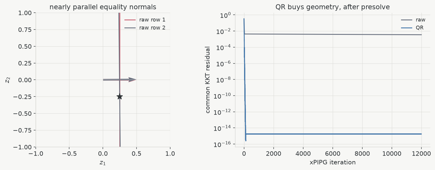
Geometrically, nearly parallel equality normals require the integral state to build very different coefficients before $H^\top w$ can move in all primal directions. QR replaces those normals by orthogonal, equally scaled ones. In the two-dimensional example below, the raw singular values are approximately $1.414$ and $0.00707$; after QR both are $2.236$. The equality-KKT condition number falls from $8.9\times10^4$ to $5$, and xPIPG reaches the target in 37 iterations where the raw representation does not reach it within 12,000.

This result is deliberately narrow. QR requires full-row-rank equalities, computes a factorization and triangular solve during presolve, and often fills in a sparse constraint matrix. It is not a structure-preserving generic conic preconditioner.

Hypersphere preconditioning and projection structure

If $P=R^\top R\succ0$, define new coordinates

The quadratic Hessian becomes the identity and the constraint operator becomes $HR^{-1}$. Cone-compatible block-row normalization can then scale equality and orthant rows individually, but every row within an SOC block must receive the same scalar so that the cone itself is preserved.

The primal set becomes

This is the decisive qualification. If $D$ is a box and $R$ is a general dense matrix, $RD$ is a rotated parallelotope. Componentwise clipping is no longer its Euclidean projection. Whitening has improved the Hessian while destroying the inexpensive primal operator that made PIPG attractive. Diagonal or suitable block-diagonal Hessians can avoid this conflict; an arbitrary Cholesky factor cannot.

After compatible whitening and row normalization, the newer preconditioning paper also chooses an objective scalar. If $\sigma_{\min}=\lambda_{\min}(\widehat H\widehat H^\top)$, the derived scale is

and the corresponding PIPG ratio is written as

Objective scaling and the primal–dual step ratio therefore describe the same relative degree of freedom in this construction; they should not be tuned as if they were independent.

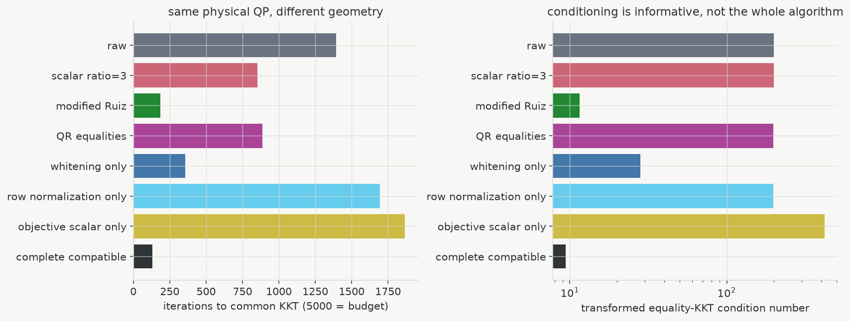
The following experiment writes one trajectory QP in eight mathematically equivalent representations. Scalar ratio tuning reduces 1395 iterations to 853 without changing the KKT condition number. Modified Ruiz needs 184; whitening alone needs 357; QR needs 886 and raises operator density from $0.067$ to $0.288$. The complete projection-compatible hypersphere, block-row, and objective-scale construction needs 130 iterations. These numbers are not a ranking of preconditioners in general—the QR example above already shows a regime in which QR is much stronger—but they expose why no single condition number or scalar parameter describes the whole iteration.

The practical principle is simple: a preconditioner is useful only when it improves geometry without making the required projections or operator applications more expensive than the original problem.

Per-iteration operations

The recurring work is easier to compare after separating it from setup:

The phrase “no linear-system solve” applies to the explicit online PIPG/xPIPG kernel under this representation. It does not include QR or Cholesky preconditioning, singular-value estimation, compilation, or a projection that internally solves another optimization problem. Conversely, a direct ADMM iteration reuses rather than repeats its factorization, and its triangular solves may be exceptionally efficient for a small fixed system.

Warm starts are natural for all of these fixed-point states. For ADMM one warms the primal, split, and dual variables. For xPIPG one must distinguish the relaxed states $(\xi,\eta)$ from the projected base points $(z,w)$ and transform the dual state consistently if the constraints have been scaled.

Setup cost and amortization

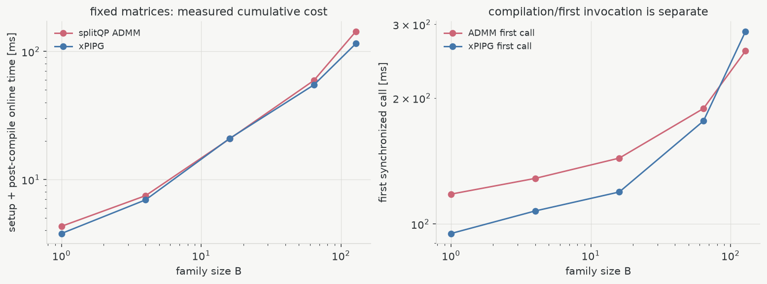
A timing comparison is meaningful only if both methods use the same physical residuals and neither is charged selectively for setup. Data construction, factorization or norm estimation, compilation, and online execution are therefore separated, and both methods stop on the same original-coordinate KKT criterion. An independent reference solution is used to check the result, not to decide when either iteration stops.

Two regimes were measured. In the changing-matrix regime, varying the dynamics time step changes $P$ or $A$ while preserving array shapes. ADMM repeats a $1.37$–$2.55$ ms setup and a $1.90$–$6.87$ ms online solve; xPIPG repeats a $0.65$–$0.72$ ms norm/step setup and a $2.57$–$3.15$ ms online solve. Both terminate at an original-coordinate KKT residual of approximately $10^{-5}$. The ranges overlap, so even this small example does not support a categorical claim.

With fixed matrices, both methods reuse setup and consecutive targets warm-start from the preceding terminal state. At family size $B=1$, post-compilation online time is about $3.1$ ms for either method; including setup gives $4.3$ ms for ADMM and $3.8$ ms for xPIPG. At $B=128$, the corresponding totals are $143.4$ ms and $115.2$ ms in this CPU experiment, although xPIPG performs 63,780 iterations against ADMM’s 33,061. Here the cheaper explicit kernel offsets a higher iteration count. A different factorization backend, sparsity pattern, accuracy target, or processor can move the crossing point.

Iteration count alone is therefore an incomplete cost model. ADMM performs triangular solves and stores a factor whose fill-in depends on the matrix ordering. PIPG performs more exposed matrix–vector products and stores only vector states beyond the operators, but may need more iterations.

Computational regimes

For a small dense QP with fixed $P$ and $A$, many nearby right-hand sides, and a factorization that fits comfortably in memory, reusable-factor ADMM is a natural choice. Its implicit primal step absorbs curvature and coupling into a well-tested linear algebra kernel, and higher accuracy can justify the work spent on that kernel.

xPIPG becomes more plausible when matrices change frequently, when $P$ and $H$ are available only as matrix-free operators, or when a large independent batch maps well to accelerators. These advantages require $D$ and $K^\circ$ to have cheap projections. If either projection is a QP, or if whitening rotates a box into a difficult set, the explicit iteration has lost the property on which the comparison depends.

Poor coordinates can make either method look ineffective. ADMM then struggles with an unbalanced penalty metric or linear system; PIPG struggles with a small stable global step and weak progress in slow directions. Preconditioning must be evaluated together with presolve cost, sparsity, projection preservation, and the number of solves over which it can be amortized.

The common structure is now visible without collapsing the algorithms into one another. ADMM, PIPG, and PDHG are primal–dual fixed-point methods in which constraint residuals update a dual-like state and a transpose operator returns constraint information to primal space. ADMM realizes its main primal update through a proximal minimization; PIPGeq and PIPG use a forward gradient and explicit PI prediction–correction. In that correction, the proportional term is the current penalty gradient and the integral term is multiplier memory. xPIPG relaxes the resulting fixed-point map and makes its displacement directions observable. Which construction is preferable is a property of the problem representation and computational regime, not of the method name alone.

The executable JAX notebook implements each displayed update directly and reproduces the figures. It uses the existing splitQP ADMM implementation as the comparison and CVXPY with Clarabel only as an independent numerical reference.

References

1. Stephen Boyd, Neal Parikh, Eric Chu, Borja Peleato, and Jonathan Eckstein. Distributed Optimization and Statistical Learning via the Alternating Direction Method of Multipliers. Foundations and Trends in Machine Learning, 3(1):1–122, 2011. paper
2. Bartolomeo Stellato, Goran Banjac, Paul Goulart, Alberto Bemporad, and Stephen Boyd. OSQP: An Operator Splitting Solver for Quadratic Programs. Mathematical Programming Computation, 12:637–672, 2020. paper
3. Yue Yu, Purnanand Elango, and Behçet Açıkmeşe. Proportional-Integral Projected Gradient Method for Model Predictive Control. arXiv:2009.06980, 2020. paper
4. Yue Yu, Purnanand Elango, Ufuk Topcu, and Behçet Açıkmeşe. Proportional-Integral Projected Gradient Method for Conic Optimization. arXiv:2108.10260, 2021. paper
5. Yue Yu and Ufuk Topcu. Proportional-Integral Projected Gradient Method for Infeasibility Detection in Conic Optimization. arXiv:2109.02756, 2021. paper
6. Yue Yu, Purnanand Elango, Behçet Açıkmeşe, and Ufuk Topcu. Extrapolated Proportional-Integral Projected Gradient Method for Conic Optimization. arXiv:2203.04188, 2022. paper
7. Govind M. Chari, Yue Yu, and Behçet Açıkmeşe. Constraint Preconditioning and Parameter Selection for a First-Order Primal-Dual Method Applied to Model Predictive Control. arXiv:2403.15656, 2024. paper
8. Abhinav G. Kamath, Purnanand Elango, and Behçet Açıkmeşe. Optimal Preconditioning for Online Quadratic Cone Programming. arXiv:2501.14191, 2025. paper

The algorithmic implementations were checked against pipg-demo, optimal-preconditioning, trajopt-util, and the secondary application-specific PIPG-Cpp implementation.

A quadratic program has a quadratic objective and linear constraints, so one might expect Newton’s method to solve it in a single step. That is almost true. After introducing slack variables, stationarity and primal feasibility are affine equations. The only nonlinear KKT equation is complementarity, \(s_i z_i=0\), and nearly all of the interesting interior-point machinery is organized around that one product.

Mehrotra’s predictor–corrector method handles it in an unusually economical way. At each iterate it first asks where an aggressive affine-scaling step would go if complementarity were driven directly to zero. That hypothetical step is not accepted. Instead, it is used twice: to choose how strongly the next direction should be centered, and to estimate the second-order term discarded by the Newton model. A second solve then corrects the model. Both solves use the same KKT matrix, so the expensive factorization is reused.

This is the main idea of the method. The rest of the article makes each part of that statement precise.

Mehrotra’s 1992 paper develops the method for linear programs. The presentation below uses the now-standard convex QP form found in CVXOPT, CVXGEN, and HPIPM. The Hessian changes the linear algebra, but the predictor–corrector mechanism still lives in complementarity.

KKT Conditions for a Convex QP

Consider the convex quadratic program

Introduce a slack \(s\in\mathbb R^m\) and dual variables \(y\) and \(z\):

The KKT residuals are

and optimality additionally requires

where \(\odot\) denotes elementwise multiplication. The first three equations are affine in the primal–dual variables. Equation (3) is the only nonlinear one.

An interior-point method avoids the boundary by keeping \(s,z\succ0\) and replacing (3) with

For feasible points, these equations describe the central path. The parameter

is the average complementarity, and \(s^\top z=m\mu\) is the surrogate duality gap. As \(\mu\) decreases, the path approaches a KKT point. Componentwise centrality matters: a small average can still hide a few badly unbalanced pairs \(s_i z_i\). This is the primal–dual version of the central-path picture developed in Chapter 11 of Convex Optimization.

The iterates of an infeasible-start method need not lie exactly on this path, or even satisfy the linear constraints. The path is a geometric guide; the algorithm works with all four residual blocks at once.

The Primal–Dual Newton System

Let \(S=\operatorname{diag}(s)\), \(Z=\operatorname{diag}(z)\), and stack the variables as \(w=(x,y,z,s)\). Linearizing the KKT equations around the current iterate gives the Jacobian

A primal–dual Newton direction toward a complementarity target \(\mu_t\) solves

Notice what does not appear in \(J\): the target \(\mu_t\). At a fixed iterate, changing the desired complementarity changes only the right-hand side. This is the computational opening exploited by the predictor–corrector method.

There is also a useful central-path interpretation. If \(w^\star(\mu)\) is exactly on the path, implicit differentiation of the perturbed KKT equations gives

A first-order prediction from the current \(\mu\) toward \(0\) therefore satisfies

Thus, on the central path, the affine-scaling direction is exactly the tangent prediction obtained by aiming at zero complementarity. Away from the path this is only the geometric intuition: the actual direction must also reduce \(r_d,r_e,r_i\). In Mehrotra’s original formulation, the broader interpretation is a local expansion of a primal–dual affine-scaling trajectory from the current positive point.

The Affine-Scaling Predictor

The predictor chooses the most aggressive possible target, \(\mu_t=0\):

If the linear model were exact and a full step remained interior, this direction would satisfy the unperturbed KKT equations in one move. Usually it heads toward the boundary. We compute the largest hypothetical step that preserves nonnegativity,

and inspect the complementarity at that affine point:

The important word is inspect. The affine point is a prediction, not the next iterate. Its job is to report how much progress the current Newton geometry appears to permit.

That report determines the centering parameter. A standard QP implementation uses

If the affine probe predicts a large reduction in complementarity, then \(\mu_{\mathrm{aff}}/\mu\) is small and so is \(\sigma\): the combined direction can remain aggressive. If the probe makes little progress, \(\sigma\) grows and pulls more strongly toward the center. The cube is a successful heuristic rather than a consequence of Newton’s method; variants of the exponent and clipping rule appear in different implementations.

This feedback is one of Mehrotra’s most useful ideas. Instead of prescribing a barrier schedule in advance, the method asks the current linearized problem how ambitious the next target should be.

The Centering-Corrector Direction

Centering alone is not the whole second solve. The exact complementarity after a step is

Newton’s method retains the two linear terms and discards the product of the directions. For the affine predictor,

so the complementarity left by a full affine step is precisely the omitted quadratic term

The predictor has therefore done more than estimate a step length. It has measured the leading error of its own linear model. Mehrotra’s corrector uses that measurement while also adding the adaptive centering target:

The two terms in the last block play different roles. The centering term \(\sigma\mu\mathbf 1\) prevents a few complementarity pairs from collapsing much faster than the others. The correction term subtracts a concrete second-order defect revealed by the affine solve.

This also clarifies a common misconception about the name predictor–corrector. It does not mean that the solver accepts an affine update and then repairs the new point. Both directions are computed at the same current iterate. Equivalently, the combined direction solves (5) with complementarity right-hand side

The correction is called second-order because it restores information from the product in (11), even though it is obtained through another linear solve.

The Reduced KKT System

The four-by-four system in (5) explains the algorithm, but a QP solver will usually eliminate \(\Delta s\) and \(\Delta z\) before factorization. For a generic right-hand side

define \(D=S^{-1}Z=\operatorname{diag}(z/s)\). Block elimination gives

The remaining directions follow from

This reduced saddle-point matrix is the numerical core of many second-order QP solvers. At one iterate, \(D\) is fixed. The affine and corrector systems change \(b_c\), not the matrix in (13), so the solver can factor the matrix once and apply the factors to two right-hand sides. The second direction is not free, but triangular back-solves are usually much cheaper than another sparse factorization.

Operationally, an iteration is now quite short: evaluate the residuals, form and factor (13), solve for the affine direction, compute \(\mu_{\mathrm{aff}}\), \(\sigma\), and the quadratic defect, solve the corrected right-hand side with the stored factors, and choose a safe step. That sequence is most of the algorithm.

The same equation also exposes a central numerical difficulty. Near a strictly complementary solution, an active constraint tends to have \(s_i\to0\) and \(z_i>0\), while an inactive one has \(z_i\to0\) and \(s_i>0\). The diagonal ratios \(z_i/s_i\) can therefore span many orders of magnitude. The mathematical path approaches the solution just as its linear algebra becomes increasingly ill-conditioned.

This is where a compact derivation stops and a production solver begins. CVXGEN combines static and dynamic regularization with iterative refinement; HPIPM adds residual checks, regularization, refinement, and structure-specific factorizations. For optimal-control QPs, the same saddle-point solve can be organized as a Riccati recursion rather than a generic sparse \(LDL^\top\) factorization. These choices change the numerical machinery, not the predictor–corrector logic.

Step Size and Termination

After combining the directions, choose the largest step that stays inside the orthant,

and take a fraction-to-the-boundary step

Some implementations use separate primal and dual step lengths; the common-step form keeps the notation compact. In either case, the affine boundary step in (8) is used to make a prediction, whereas (14) updates the actual iterate.

Positivity alone is not a stopping condition. An infeasible-start method must separately verify primal feasibility, stationarity, and complementarity, for example

A tiny gap does not imply a solved KKT system. Conversely, small primal and dual residuals do not imply complementarity. Practical solvers scale these tests relative to the problem data and add safeguards for small steps, non-finite directions, or insufficient progress.

Initialization

An infeasible-start method does not need a feasible initial point, but it does need \(s^0,z^0\succ0\). One useful QP initialization, used in the CVXOPT cone-program notes and in CVXGEN, begins with the regularized system

The second block gives provisional slacks \(\widetilde s=h-Gx^0=-\widetilde z\). Shift the primal and dual quantities independently,

using the smallest nonnegative shifts, with a modest margin, that make both vectors strictly positive. The shifts generally destroy exact primal or dual feasibility, which is acceptable: the residuals in (2) are already part of the Newton system.

This initialization is not part of the essential Mehrotra correction, nor is it meant to guess the optimizer. It simply creates a symmetric, numerically moderate point from which the infeasible-start iteration can begin. Different solvers use different starting strategies.

Extension to Conic Constraints

Ordinary QP inequalities are already conic constraints over the nonnegative orthant. Replacing that orthant by a second-order or positive-semidefinite cone changes the geometry of complementarity, but not the overall organization of the method.

For a cone \(K\), a logarithmically homogeneous barrier \(f\), a primal slack \(s\in K\), and a dual variable \(z\in K^\ast\), centrality can be written as

For symmetric cones—nonnegative orthants, second-order cones, and positive-semidefinite cones—this becomes

where \(\circ\) is the cone’s Jordan product and \(e\) its identity. The orthant recovers elementwise multiplication. A second-order cone instead couples a whole vector block, so componentwise positivity becomes cone interiority and the diagonal scaling in (13) becomes a cone-scaling block.

The corrector survives, but it must be written in the right coordinates. With Nesterov–Todd scaling \(W\), the symmetric-cone analogue of the quadratic defect has the form

For nonsymmetric cones such as exponential and power cones, there is no Jordan algebra and this formula does not apply; solvers such as Clarabel use barrier derivatives and a different higher-order correction. The durable idea is not a particular elementwise product. It is to use an aggressive affine solve to estimate both the attainable progress and the nonlinear defect, then reuse the same local KKT geometry for a corrected direction.

Summary

Under the hood, a second-order QP solver is not repeatedly solving a new optimization problem from scratch. It maintains an interior primal–dual state, forms one local KKT geometry, probes that geometry with a target of zero complementarity, lets the probe choose the centering strength, corrects the nonlinear term that the local model omitted, and then takes the largest safe step. Most of the time is spent factoring a structured indefinite matrix; much of solver design is about making that factorization reliable as the central path becomes ill-conditioned.

That is why Mehrotra’s method is more than “two Newton steps.” The first solve is an experiment. The second uses what the experiment revealed while the expensive linear algebra is still available. This predictor–corrector pattern appears, with different scaling and safeguards, in QP solvers such as CVXGEN, qpSWIFT, and HPIPM, and continues into modern conic solvers.

For a compact executable version of the QP equations above, see barrierQP.

References

1. S. Mehrotra, On the Implementation of a Primal-Dual Interior Point Method, SIAM Journal on Optimization, 2(4):575–601, 1992.

2. S. Boyd and L. Vandenberghe, Convex Optimization, Chapter 11, Cambridge University Press, 2004.

3. L. Vandenberghe, The CVXOPT Linear and Quadratic Cone Program Solvers, 2010.

4. J. Mattingley and S. Boyd, CVXGEN: A Code Generator for Embedded Convex Optimization, Optimization and Engineering, 13(1):1–27, 2012.

5. G. Frison and M. Diehl, HPIPM: A High-Performance Quadratic Programming Framework for Model Predictive Control, arXiv:2003.02547, 2020.

6. A. G. Pandala, Y. Ding, and H.-W. Park, qpSWIFT: A Real-Time Sparse Quadratic Program Solver for Robotic Applications, IEEE Robotics and Automation Letters, 4(4):3355–3362, 2019.

7. P. J. Goulart and Y. Chen, Clarabel: An Interior-Point Solver for Conic Programs with Quadratic Objectives, arXiv:2405.12762, 2024.

Fixed-wing perching is a canonical underactuated problem: a small glider must enter a strongly nonlinear post-stall regime, shed most of its kinetic energy in under a second, and still reach a small perch. This post asks how a deliberately simple model becomes useful enough to plan and control that maneuver.

Physics supplies coordinates and candidate terms. Data then selects compact nonlinear dynamics, corrects a flat-plate prior, and estimates drifting parameters. Direct collocation or iLQR plans, feedback tracks, and execution refines the model; CEM and a minimal MPPI implementation provide a gradient-free comparison. The model is judged by rollout and task performance, not by global fidelity.

Code: 10-trajopt/perching, with the companion glider_sysid.ipynb.

Can a fixed-wing aircraft land on a perch the way a bird does? Conventional aircraft are designed to avoid stall: they maintain attached flow, dissipate energy gradually, and rely on a runway to complete the landing. A perching bird uses a fundamentally different strategy. It pitches up aggressively, enters a post-stall regime, generates large aerodynamic drag, and nevertheless lands with remarkable precision.

That contrast is what makes fixed-wing perching an interesting underactuated control problem. The objective is not merely to reduce speed, but to shed kinetic energy rapidly while retaining enough control authority to reach a small terminal target. To study it in its simplest form, Underactuated Robotics considers a planar glider with no propeller, flat-plate wings, a single actuated tail, and enough dihedral that roll stays mostly passive. The control input is simply $u=\dot{\phi}$, the elevator rate.

The central difficulty is that the aerodynamic forces providing both drag and control authority vanish as the vehicle slows down:

If the glider pitches up too early, it bleeds energy too fast and falls short. Too late, and it overshoots. Successful perching therefore requires a sub-second coordination of kinetic energy, pitch attitude, drag, altitude, and terminal geometry — and the controller has the least authority exactly when the terminal geometry matters most. The maneuver is shown in this lecture excerpt.

A model that is wrong in the right way

The longitudinal state and input are

with $x,z$ the center-of-mass position, $\theta$ the body pitch, and $\phi$ the elevator angle. The input is elevator rate because a small hobby servo is much closer to a velocity-controlled device than to an ideal torque source.

The flat-plate prior says the dominant force on each surface acts normal to the plate and scales with dynamic pressure. For a surface with area $S$, normal $\boldsymbol{n}$, and local relative velocity $\boldsymbol{v}$,

which resolves into the familiar sines-and-cosines coefficients

where $\alpha$ is the angle of attack. Wing and elevator each carry a center-of-pressure offset from the center of mass, so the local velocity at each surface mixes translation and rotation; the two normal forces produce net force and pitch torque. The result is

with $\boldsymbol{\beta}$ collecting mass, inertia, surface areas, center-of-pressure offsets, and air density. The full derivation is in [1].

A flat plate is a poor airfoil, but it remains a useful prior in the post-stall regime because:

• the force scaling with $\rho S|\boldsymbol{v}|^2$ and the geometric coupling between pitch, elevator, and moment arm are structurally correct;
• the model is low-dimensional, smooth, and differentiable, so it can live inside a trajectory optimizer and a Riccati equation;
• with the mechanics already accounted for, data can learn the aerodynamic discrepancy instead of the full vehicle dynamics.

The same physics can also organize a compact model identified directly from data.

System identification: what should the data learn?

The real glider has a fuselage, finite wing geometry, a tail, mounting hardware, flexibility, actuator delay, and separated flow. “Learn the dynamics” can therefore mean three different things:

• a compact, physically inspired basis model asks which nonlinear terms belong in each acceleration equation;
• a flat-plate-plus-residual model trusts the mechanical backbone and asks the data only for corrections to lift, drag, and pitching moment;
• an augmented-state parameter model trusts the functional form and updates only a few physical numbers online.

Each step makes a stronger structural assumption. It needs less data, but it can correct fewer kinds of error.

1. Model structure: which nonlinear terms belong? The glider_sysid.ipynb exercise makes the weakest of these assumptions: each acceleration is a short linear combination of nonlinear, physically motivated features, but the relevant features are initially unknown:

The nonlinearity lives in the fixed feature functions $\varphi_j$; the unknown coefficients $\beta_j^r$ enter linearly. This is the same useful separation emphasized in the system-identification notes [5]: a nonlinear mechanical model can still produce a linear regression problem when its unknowns enter affinely.

The notebook uses synthetic data. TrueDynamics implements the flat-plate equations and generates 15 trajectories of 0.5 seconds each with $\Delta t=0.01$ s. Every launch begins near

with uniform perturbations on all seven states. Each rollout also receives a perturbed version of the same 50-sample elevator-rate sequence. Trajectories 1–14 provide $14\times50=700$ fitting samples; trajectory 0 is held out for forward simulation. Perturbing both state and input improves excitation, whereas repeated deterministic rollouts would only duplicate rows of the data matrix.

In the corresponding flight experiment, the glider was launched at roughly 6 m/s in a Vicon arena. Pose was recorded at 120 Hz, the elevator was commanded at 50 Hz, and the pose data were filtered acausally before being differentiated twice. A separately identified second-order elevator model included about 28 ms of delay [6]. The exercise instead uses exact simulated derivatives and treats $u=\dot\phi$ directly, isolating model selection from signal processing and actuator identification.

Before regression, the code makes a consequential coordinate choice. It removes gravity and rotates world-frame accelerations into axes tangential and normal to the wing:

This is not cosmetic preprocessing. In world coordinates the same aerodynamic force moves between $x$ and $z$ as the aircraft rotates. In the plane frame, normal and tangential effects are more nearly decoupled, so a short feature list has a chance to describe each target. Choosing a representation in which the physics is sparse is already part of system identification.

The candidate features are built from the wing speed and angle of attack $(V,\alpha)$, the elevator speed and angle of attack $(V_{el},\alpha_{el})$, pitch rate $\dot\theta$, elevator angle $\phi$, and elevator rate $u$. The notebook implements 20 features drawn from the 41-term library in Hoburg and Tedrake [6], then evaluates ten preassembled configurations. For one acceleration component and one candidate subset $s$, its design matrix is

and the fitted coefficients minimize the instantaneous equation error:

The exercise asks for the normal equation. Its implementation avoids forming the inverse explicitly,

beta = np.linalg.solve(Phi.T @ Phi, Phi.T @ y)

but the normal equation still squares the condition number of $\boldsymbol{\Phi}$. With measured data, QR/SVD through np.linalg.lstsq, a rank and singular-value check, and possibly ridge regularization are safer. A low residual cannot identify directions the experiment never excited.

Configuration 6 has the lowest summed training residual in this exercise, $63{,}831$, compared with $96{,}418$ for the next-best configuration. Written out from the actual notebook functions, it is

This is the winner among the notebook’s ten candidates, not the real-flight model reported in the paper; their data, candidate sets, and selection procedures differ.

BasisDynamics then closes the loop in the modeling pipeline. It recomputes $(V,\alpha,V_{el},\alpha_{el})$ from a state, evaluates the selected features, converts the three fitted plane-frame accelerations back to the world frame, restores gravity, fills the four kinematic derivatives, and advances the state with explicit Euler. Running that learned model from the held-out initial condition under the held-out elevator tape produces the orange rollout below.

That last step changes the question. Least squares scored instantaneous acceleration errors at observed states; forward simulation uses each predicted state to evaluate the next step. Small local biases can therefore accumulate, move the model off the data manifold, and produce a large simulation error:

The notebook uses the held-out rollout only as a diagnostic. The original work went one step further: it initialized from the linear least-squares solution and differentiated through the rollout with BPTT or RTRL to reduce simulation error directly [6]. This is why “best instantaneous fit” and “best dynamics for control” are not synonyms.

Four practical rules follow:

• Split by trajectory. Neighboring samples are correlated, so a random row split leaks nearly the same flight into training and validation.
• Check excitation and conditioning. Full rank is only the minimum; inspect singular values and excite pitch, elevator motion, and post-stall angles within the safe envelope.
• Choose complexity by held-out rollout. Extra features always reduce training residual but can destabilize simulation and controller linearizations.
• Weight the task-relevant channels. fit_score mixes translational and angular residuals with different units. Normalize or weight them, then report equation error, rollout error, and closed-loop performance separately.

System identification is therefore not finished when a regressor returns coefficients; the model must survive the rollout and controller for which it was built.

2. Residual function: how is the flat plate wrong? The basis exercise identifies a stand-alone acceleration model. The perching code makes a stronger assumption: keep the flat-plate dynamics and learn only corrections to its aerodynamic coefficients. Write

where $\boldsymbol{\psi}$ stacks Gaussian radial basis functions on a grid of centers over $(\alpha,\phi)$, plus a constant term. The weights come from ridge regression,

with $\boldsymbol{\Phi}$ the design matrix whose rows are $\boldsymbol{\psi}(\xi_n)^{\top}$. The model is nonlinear in the flight condition and linear in the unknowns, so identification is a single regularized linear solve — no local minima, no rollout differentiation.

These are Gaussian radial basis functions, not a Gaussian process. They form a fixed, finite feature map whose coefficients are point estimates; there is no kernel posterior or predictive covariance. The ME696 notes make the same distinction [4].

The repository’s coefficient dataset contains roughly $3.9\times10^{3}$ samples of $(\alpha,\phi,V,\dot\alpha,\dot\theta)$ with corresponding $C_L$, $C_D$, and $C_M$, plus a flat-plate baseline at the same conditions. In the experimental pipeline developed further in Moore’s thesis, about 50 launches spanned initial speeds from 6 to 8 m/s. Position measurements were filtered, differentiated twice, and compared with flat-plate predictions before fitting residual lift, drag, and moment coefficients [7]. The learner therefore models a smaller target in the part of the flight envelope relevant to perching.

Two implementations use this idea at different scopes:

• the standalone fitting example (fit_coeffs.m) fits only the lift residual, on a $5\times5$ grid of centers over $(\alpha,\phi)$ plus a bias — 26 weights — and compares the result against the stored coefficient model;
• the model-learning script parameterizes and identifies residuals for lift, drag, and pitching moment with the same feature construction, 26 weights each.

The first plot shows the flat-plate backbone bent toward the data by the fitted residual; the second overlays the stored model. Feature grids, regularization, and preprocessing can change the exact curve, but both retain a compact correction on a physical baseline.

3. Physical parameters: which numbers drift? Some mismatch is a wrong number rather than a wrong function: a repair can shift the center of pressure, and effective control-surface area need not match the drawing. For a small parameter set,

the natural move is to stop treating them as constants and start treating them as slow states. Augment,

and run an EKF on $\bar{\boldsymbol{x}}$. The implementation measures the full physical state ($\boldsymbol{H}=[\,\boldsymbol{I}\;\;\boldsymbol{0}\,]$, mocap-style), gives the filter the current wind, and asks it only for the two aerodynamic parameters.

Nothing measures $l_w$ or $S_e$ directly. They are inferred because parameter errors change accelerations and therefore the filter innovation. Without pitch change, elevator motion, or high angle of attack, that innovation carries little information about them. Excitation determines identifiability.

In this demonstration, an infinite-horizon LQR holds the vehicle near cruise while simulated wind drifts, so excitation comes only from disturbance rejection. A perch would be more informative because its large pitch excursion, elevator motion, and post-stall angles make these parameters more observable.

Together, residual learning and parameter estimation provide the data-corrected state-space model used by the planner and controller below.

Planning the maneuver, and protecting it

Forward simulation asks what happens if we replay a chosen input. Trajectory optimization asks the inverse question: does there exist any dynamically consistent motion from the launch state to the perch? Rather than choosing inputs and integrating forward in time order, direct collocation lets the optimizer choose state and input samples together, then constrains the interpolating curve to satisfy the differential equation at collocation points [1].

The notebook does four things, in order:

1. Solve for a nominal trajectory by direct collocation. The launch state is fixed ($x=-3.5$ m, $z=0.1$ m, $\dot x=7$ m/s); the terminal state is pinned to the perch in position with bounded pitch and bounded terminal velocity; elevator angle and elevator rate carry servo limits; there is a running cost on input effort and a terminal quadratic error cost pulling pitch toward $-\pi/4$. Nothing in the problem says pitch up here, stall here, catch the perch here. The timing is discovered.
2. Warm-start a finer mesh from a coarser one. The same program is solved at 25 knot points and then re-solved at 41, seeded by the first solution. The finer problem therefore starts near a feasible maneuver rather than from a fresh interpolated guess.
3. Replay the nominal input open-loop and watch the trajectory drift away from the plan.
4. Wrap the nominal in finite-horizon LQR and re-simulate from several perturbed initial conditions (the launch height is jittered), using the time-varying gain to correct the tracking error $\boldsymbol{x}(t)-\boldsymbol{x}_0(t)$:

The Riccati derivation behind $\boldsymbol{K}(t)$ is standard and lives in [2]. Open-loop replay is the experiment that justifies feedback: dynamics were enforced only at finitely many collocation points, forward integration does not exactly reproduce the transcription, and the maneuver is sensitive. Hardware would add model error on top of that numerical drift.

The division of labor is clean, and it is the reason both pieces are here:

Trajectory optimization finds a feasible schedule for throwing away energy. Finite-horizon LQR defends a neighborhood of that schedule. One answers how should it fly; the other answers if it drifts, can it get back.

The controller is not stabilizing a fixed point but a moving reference, and its authority decays along the way — the maneuver deliberately destroys the dynamic pressure on which control effectiveness depends. In perching that fragility is concentrated near the end, where the terminal geometry is least forgiving.

A note on funnels

A closed-loop rollout is an example: this initial condition worked. The stronger statement is a funnel — a time-varying set $\mathcal{F}(t)$ such that every state inside it at time $t$ is driven to the target set at $t_f$. The usual construction takes the LQR cost-to-go as a Lyapunov candidate, $V(t,\bar{\boldsymbol{x}})=\bar{\boldsymbol{x}}^{\top}\boldsymbol{S}(t)\bar{\boldsymbol{x}}$ with $\bar{\boldsymbol{x}}=\boldsymbol{x}-\boldsymbol{x}_0(t)$, picks a terminal sublevel set inside the acceptable perching set, and integrates backward while requiring the closed-loop vector field to point inward on the boundary. Verifying that condition over a continuum of states is the hard part; sums-of-squares programming with the $S$-procedure turns it into a tractable sufficient certificate. Underactuated develops both the funnel construction and the SOS machinery [1], [3].

The notebook stops at closed-loop simulation from sampled initial conditions. The SOS script in the same directory instead studies the region of attraction of a reversed Van der Pol oscillator, using bilinear alternation between a multiplier step and a $\rho$-maximization step. A perching funnel is therefore a next step rather than a result of this repository; the figure below comes from the experimental work.

Even when it is not computed, the funnel names the relevant quantity: its width measures how much deviation the closed loop can recover. Shrinking near the perch reflects the loss of control authority in low-speed post-stall flight.

Closing the loop: improving the model the planner uses

So far learning happened before planning. The model-learning script puts it inside the loop: use the current model to plan, execute with local feedback, measure the model error, refit, and plan again.

This is deterministic, structured model-based learning: the controller improves because the point-estimate model it plans through improves. Unlike PILCO, it carries no GP posterior or predictive covariance through the horizon [4].

The planner integrates

where $f_{\mathrm{fp}}$ is the flat-plate model and the columns of $\boldsymbol{G}$ are the RBF features scaled by dynamic pressure and resolved into the lift, drag, and moment directions — so $\boldsymbol{G}\boldsymbol{w}$ is exactly the aerodynamic correction, and the dynamics are affine in the unknowns. The weights start at zero, which means iteration 0 plans through pure flat-plate physics.

Plan. iLQR is used as a fast local optimizer for the current model, returning a nominal maneuver and a time-varying affine policy. Its forward pass rolls out an improved nominal using the feedforward step and a backtracking line search; [1] gives the standard backward pass.

Execute. The feedforward term $\boldsymbol{k}$ is a planning object: the iLQR forward pass uses it to update the nominal control sequence. Execution therefore uses the updated nominal plus local feedback,

with the launch speed randomized each iteration so successive rollouts are not identical.

Identify. Finite differences on the executed rollout give $\dot{\boldsymbol{x}}{\mathrm{data},n}\approx(\boldsymbol{x}{n+1}-\boldsymbol{x}_n)/h$, and because the residual enters affinely, the update is again a ridge least-squares solve — restricted to the three components where the aerodynamic residual acts directly:

Here $\boldsymbol{\Pi}_a$ selects $(\ddot x,\ddot z,\ddot\theta)$; the remaining four equations are kinematic and carry no information about $\boldsymbol{w}$. Rollouts accumulate, so each solve is a batch fit over the full history rather than over the latest flight alone.

A deliberate mismatch tests the method: the planner’s residual features depend on $(\alpha,\phi)$ — 26 weights per coefficient — while the simulator uses $(\alpha,\phi,V)$ on a finer grid — 126 weights per coefficient. Airspeed dependence is structurally unavailable to the planner. No amount of data can make $\boldsymbol{w}$ represent it.

The loop therefore converges not to the simulator dynamics, but to the best flat-plate-plus-$(\alpha,\phi)$ residual along the states visited by this maneuver. That can be sufficient for replanning. The weight-change plot diagnoses convergence of the fit, while executed terminal cost measures task-relevant improvement.

Two caveats bound the plots: finite differencing amplifies the noise added to measured states, and randomized launch speed makes some terminal-cost variation attributable to the initial condition rather than the model.

Without gradients: CEM and a minimal MPPI-style optimizer

Direct collocation and iLQR exploit derivatives of the dynamics or cost. A separate script includes two sampling-based alternatives that share a rollout function, cost, and horizon.

Both methods optimize one open-loop control sequence $\boldsymbol{U}={u_0,\dots,u_{N-1}}$ over a fixed $0.75$ s horizon and roll candidates through the nonlinear glider model with explicit Euler. The horizon is never shifted and the measured state never triggers replanning, so this is offline sampling-based trajectory optimization, not MPC.

CEM keeps a per-timestep Gaussian over $u_k$ with diagonal variance. Each iteration draws 30 rollouts, keeps the 10 cheapest, and re-estimates the mean and variance by maximum likelihood on that elite set, with a floor on the variance so exploration cannot collapse. It is the cross-entropy idea specialized to a control sequence: refit the sampling distribution to the good samples and repeat.

MPPI keeps a single nominal sequence and perturbs it, $u^{(r)}_k=u_k+\epsilon^{(r)}_k$ with $\epsilon^{(r)}_k$ i.i.d. Gaussian. Rather than a single score per rollout, the implementation forms a time-indexed cost-to-go

turns it into a softmax at each time step,

and moves the nominal by the weighted average of the perturbations,

This is a minimal MPPI-style optimizer. Canonical MPPI adds likelihood-ratio terms to a modified rollout cost and applies the update in a receding-horizon loop; both are absent here [8]. The ME696 notes derive the update from the stochastic HJB equation [4], while [9] gives a KL-regularized interpretation. Numerically, subtracting the minimum cost before exponentiation would preserve the normalized weights while avoiding underflow.

Four details determine how to read the result:

• $\lambda$ controls selection pressure. Small values approach the best sampled rollout; large values approach an unweighted average.
• Perturbation covariance defines the search geometry. It decides whether the samples can reach useful regions of control-sequence space.
• The time-indexed weights are nearly degenerate here. Running cost contains only a small control penalty, while terminal position and pitch dominate. Consequently $S_k^{(r)}$ changes little with $k$ and the update behaves almost like one weight per rollout.
• Search noise is not robustness. The perturbations model neither wind, sensor error, nor aerodynamic uncertainty. Robustness would require sampling those uncertainties or repeatedly replanning from measurements.

With the same horizon, dynamics, cost, and 30 rollouts per iteration, MPPI descends faster early in this run while CEM improves more evenly and ends at a comparable cost. The methods were not tuned against each other, and their parameters are not commensurate, so this is one observation rather than a ranking.

Across the identification and control pipeline, the useful hierarchy is the same: equation-error fitting can initialize a model, held-out simulation tests whether local errors accumulate, and closed-loop task performance decides whether the model is adequate. Complexity should be added only when the data can identify it and the planner can use it. Perching succeeds because physics, data, optimization, and feedback make the remaining local model error manageable.

References

[1] Russ Tedrake. Underactuated Robotics: Trajectory Optimization. Online course notes. [link]

[2] Russ Tedrake. Underactuated Robotics: Linear Quadratic Regulators — finite-horizon LQR. Online course notes. [link]

[3] Russ Tedrake. Underactuated Robotics: Lyapunov analysis with convex optimization. Online course notes. [link]

[4] Joseph Moore. Learning-Based Control for Robotics. Course notes for JHU ME696, 2025. [link]

[5] Russ Tedrake. Underactuated Robotics: System Identification. Online course notes. [link]

[6] Warren Hoburg and Russ Tedrake. System Identification of Post Stall Aerodynamics for UAV Perching. AIAA Infotech@Aerospace Conference, Seattle, Washington, 2009. [link]

[7] Joseph Moore. Robust Post-Stall Perching with a Fixed-Wing UAV. PhD thesis, Massachusetts Institute of Technology, September 2014. [link]

[8] Grady Williams, Andrew Aldrich, and Evangelos A. Theodorou. Model Predictive Path Integral Control: From Theory to Parallel Computation. Journal of Guidance, Control, and Dynamics, 40(2):344–357, 2017. [link]

[9] Heng Yang. Optimal Control and Reinforcement Learning, Ch. 4: Model-Based Planning and Optimization. Textbook for Harvard ES/AM 158, 2025. [link]