Model-Based Fixed-Wing Perching

TL;DR

Fixed-wing perching is a canonical underactuated problem: a small glider must enter a strongly nonlinear post-stall regime, shed most of its kinetic energy in under a second, and still reach a small perch. This post asks how a deliberately simple model becomes useful enough to plan and control that maneuver.

Physics supplies coordinates and candidate terms. Data then selects compact nonlinear dynamics, corrects a flat-plate prior, and estimates drifting parameters. Direct collocation or iLQR plans, feedback tracks, and execution refines the model; CEM and a minimal MPPI implementation provide a gradient-free comparison. The model is judged by rollout and task performance, not by global fidelity.

Code: 10-trajopt/perching, with the companion glider_sysid.ipynb.

Can a fixed-wing aircraft land on a perch the way a bird does? Conventional aircraft are designed to avoid stall: they maintain attached flow, dissipate energy gradually, and rely on a runway to complete the landing. A perching bird uses a fundamentally different strategy. It pitches up aggressively, enters a post-stall regime, generates large aerodynamic drag, and nevertheless lands with remarkable precision.

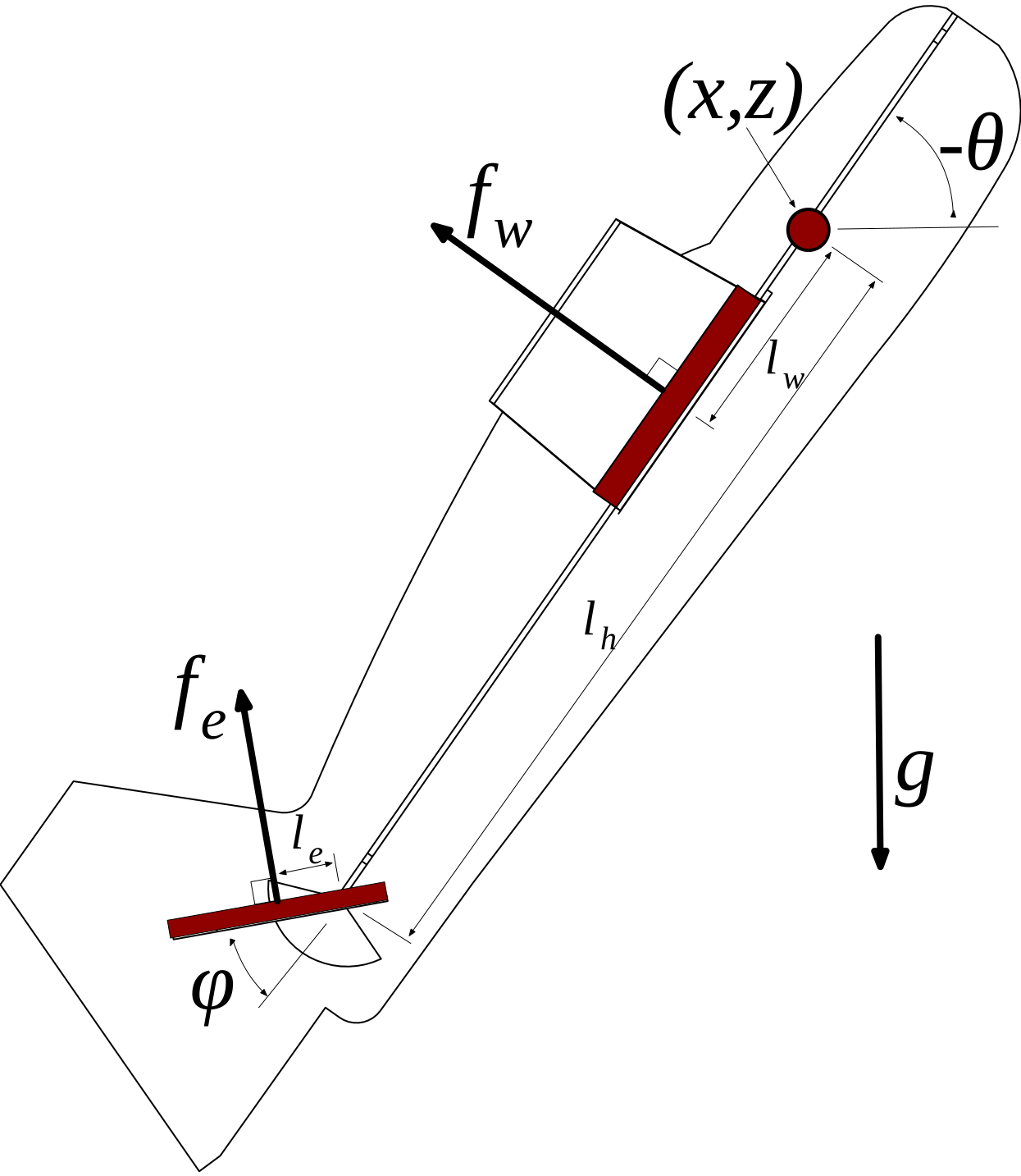
That contrast is what makes fixed-wing perching an interesting underactuated control problem. The objective is not merely to reduce speed, but to shed kinetic energy rapidly while retaining enough control authority to reach a small terminal target. To study it in its simplest form, Underactuated Robotics considers a planar glider with no propeller, flat-plate wings, a single actuated tail, and enough dihedral that roll stays mostly passive. The control input is simply $u=\dot{\phi}$, the elevator rate.

The central difficulty is that the aerodynamic forces providing both drag and control authority vanish as the vehicle slows down:

If the glider pitches up too early, it bleeds energy too fast and falls short. Too late, and it overshoots. Successful perching therefore requires a sub-second coordination of kinetic energy, pitch attitude, drag, altitude, and terminal geometry — and the controller has the least authority exactly when the terminal geometry matters most. The maneuver is shown in this lecture excerpt.

A model that is wrong in the right way

The longitudinal state and input are

with $x,z$ the center-of-mass position, $\theta$ the body pitch, and $\phi$ the elevator angle. The input is elevator rate because a small hobby servo is much closer to a velocity-controlled device than to an ideal torque source.

The flat-plate prior says the dominant force on each surface acts normal to the plate and scales with dynamic pressure. For a surface with area $S$, normal $\boldsymbol{n}$, and local relative velocity $\boldsymbol{v}$,

which resolves into the familiar sines-and-cosines coefficients

where $\alpha$ is the angle of attack. Wing and elevator each carry a center-of-pressure offset from the center of mass, so the local velocity at each surface mixes translation and rotation; the two normal forces produce net force and pitch torque. The result is

with $\boldsymbol{\beta}$ collecting mass, inertia, surface areas, center-of-pressure offsets, and air density. The full derivation is in [1].

A flat plate is a poor airfoil, but it remains a useful prior in the post-stall regime because:

• the force scaling with $\rho S|\boldsymbol{v}|^2$ and the geometric coupling between pitch, elevator, and moment arm are structurally correct;
• the model is low-dimensional, smooth, and differentiable, so it can live inside a trajectory optimizer and a Riccati equation;
• with the mechanics already accounted for, data can learn the aerodynamic discrepancy instead of the full vehicle dynamics.

The same physics can also organize a compact model identified directly from data.

System identification: what should the data learn?

The real glider has a fuselage, finite wing geometry, a tail, mounting hardware, flexibility, actuator delay, and separated flow. “Learn the dynamics” can therefore mean three different things:

• a compact, physically inspired basis model asks which nonlinear terms belong in each acceleration equation;
• a flat-plate-plus-residual model trusts the mechanical backbone and asks the data only for corrections to lift, drag, and pitching moment;
• an augmented-state parameter model trusts the functional form and updates only a few physical numbers online.

Each step makes a stronger structural assumption. It needs less data, but it can correct fewer kinds of error.

1. Model structure: which nonlinear terms belong? The glider_sysid.ipynb exercise makes the weakest of these assumptions: each acceleration is a short linear combination of nonlinear, physically motivated features, but the relevant features are initially unknown:

The nonlinearity lives in the fixed feature functions $\varphi_j$; the unknown coefficients $\beta_j^r$ enter linearly. This is the same useful separation emphasized in the system-identification notes [5]: a nonlinear mechanical model can still produce a linear regression problem when its unknowns enter affinely.

The notebook uses synthetic data. TrueDynamics implements the flat-plate equations and generates 15 trajectories of 0.5 seconds each with $\Delta t=0.01$ s. Every launch begins near

with uniform perturbations on all seven states. Each rollout also receives a perturbed version of the same 50-sample elevator-rate sequence. Trajectories 1–14 provide $14\times50=700$ fitting samples; trajectory 0 is held out for forward simulation. Perturbing both state and input improves excitation, whereas repeated deterministic rollouts would only duplicate rows of the data matrix.

In the corresponding flight experiment, the glider was launched at roughly 6 m/s in a Vicon arena. Pose was recorded at 120 Hz, the elevator was commanded at 50 Hz, and the pose data were filtered acausally before being differentiated twice. A separately identified second-order elevator model included about 28 ms of delay [6]. The exercise instead uses exact simulated derivatives and treats $u=\dot\phi$ directly, isolating model selection from signal processing and actuator identification.

Before regression, the code makes a consequential coordinate choice. It removes gravity and rotates world-frame accelerations into axes tangential and normal to the wing:

This is not cosmetic preprocessing. In world coordinates the same aerodynamic force moves between $x$ and $z$ as the aircraft rotates. In the plane frame, normal and tangential effects are more nearly decoupled, so a short feature list has a chance to describe each target. Choosing a representation in which the physics is sparse is already part of system identification.

The candidate features are built from the wing speed and angle of attack $(V,\alpha)$, the elevator speed and angle of attack $(V_{el},\alpha_{el})$, pitch rate $\dot\theta$, elevator angle $\phi$, and elevator rate $u$. The notebook implements 20 features drawn from the 41-term library in Hoburg and Tedrake [6], then evaluates ten preassembled configurations. For one acceleration component and one candidate subset $s$, its design matrix is

and the fitted coefficients minimize the instantaneous equation error:

The exercise asks for the normal equation. Its implementation avoids forming the inverse explicitly,

beta = np.linalg.solve(Phi.T @ Phi, Phi.T @ y)

but the normal equation still squares the condition number of $\boldsymbol{\Phi}$. With measured data, QR/SVD through np.linalg.lstsq, a rank and singular-value check, and possibly ridge regularization are safer. A low residual cannot identify directions the experiment never excited.

Configuration 6 has the lowest summed training residual in this exercise, $63{,}831$, compared with $96{,}418$ for the next-best configuration. Written out from the actual notebook functions, it is

This is the winner among the notebook’s ten candidates, not the real-flight model reported in the paper; their data, candidate sets, and selection procedures differ.

BasisDynamics then closes the loop in the modeling pipeline. It recomputes $(V,\alpha,V_{el},\alpha_{el})$ from a state, evaluates the selected features, converts the three fitted plane-frame accelerations back to the world frame, restores gravity, fills the four kinematic derivatives, and advances the state with explicit Euler. Running that learned model from the held-out initial condition under the held-out elevator tape produces the orange rollout below.

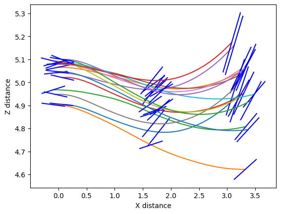
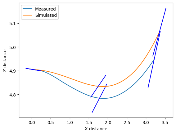
That last step changes the question. Least squares scored instantaneous acceleration errors at observed states; forward simulation uses each predicted state to evaluate the next step. Small local biases can therefore accumulate, move the model off the data manifold, and produce a large simulation error:

The notebook uses the held-out rollout only as a diagnostic. The original work went one step further: it initialized from the linear least-squares solution and differentiated through the rollout with BPTT or RTRL to reduce simulation error directly [6]. This is why “best instantaneous fit” and “best dynamics for control” are not synonyms.

Four practical rules follow:

• Split by trajectory. Neighboring samples are correlated, so a random row split leaks nearly the same flight into training and validation.
• Check excitation and conditioning. Full rank is only the minimum; inspect singular values and excite pitch, elevator motion, and post-stall angles within the safe envelope.
• Choose complexity by held-out rollout. Extra features always reduce training residual but can destabilize simulation and controller linearizations.
• Weight the task-relevant channels. fit_score mixes translational and angular residuals with different units. Normalize or weight them, then report equation error, rollout error, and closed-loop performance separately.

System identification is therefore not finished when a regressor returns coefficients; the model must survive the rollout and controller for which it was built.

2. Residual function: how is the flat plate wrong? The basis exercise identifies a stand-alone acceleration model. The perching code makes a stronger assumption: keep the flat-plate dynamics and learn only corrections to its aerodynamic coefficients. Write

where $\boldsymbol{\psi}$ stacks Gaussian radial basis functions on a grid of centers over $(\alpha,\phi)$, plus a constant term. The weights come from ridge regression,

with $\boldsymbol{\Phi}$ the design matrix whose rows are $\boldsymbol{\psi}(\xi_n)^{\top}$. The model is nonlinear in the flight condition and linear in the unknowns, so identification is a single regularized linear solve — no local minima, no rollout differentiation.

These are Gaussian radial basis functions, not a Gaussian process. They form a fixed, finite feature map whose coefficients are point estimates; there is no kernel posterior or predictive covariance. The ME696 notes make the same distinction [4].

The repository’s coefficient dataset contains roughly $3.9\times10^{3}$ samples of $(\alpha,\phi,V,\dot\alpha,\dot\theta)$ with corresponding $C_L$, $C_D$, and $C_M$, plus a flat-plate baseline at the same conditions. In the experimental pipeline developed further in Moore’s thesis, about 50 launches spanned initial speeds from 6 to 8 m/s. Position measurements were filtered, differentiated twice, and compared with flat-plate predictions before fitting residual lift, drag, and moment coefficients [7]. The learner therefore models a smaller target in the part of the flight envelope relevant to perching.

Two implementations use this idea at different scopes:

• the standalone fitting example (fit_coeffs.m) fits only the lift residual, on a $5\times5$ grid of centers over $(\alpha,\phi)$ plus a bias — 26 weights — and compares the result against the stored coefficient model;
• the model-learning script parameterizes and identifies residuals for lift, drag, and pitching moment with the same feature construction, 26 weights each.

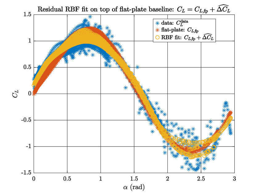
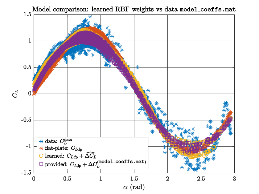
The first plot shows the flat-plate backbone bent toward the data by the fitted residual; the second overlays the stored model. Feature grids, regularization, and preprocessing can change the exact curve, but both retain a compact correction on a physical baseline.

3. Physical parameters: which numbers drift? Some mismatch is a wrong number rather than a wrong function: a repair can shift the center of pressure, and effective control-surface area need not match the drawing. For a small parameter set,

the natural move is to stop treating them as constants and start treating them as slow states. Augment,

and run an EKF on $\bar{\boldsymbol{x}}$. The implementation measures the full physical state ($\boldsymbol{H}=[\,\boldsymbol{I}\;\;\boldsymbol{0}\,]$, mocap-style), gives the filter the current wind, and asks it only for the two aerodynamic parameters.

Nothing measures $l_w$ or $S_e$ directly. They are inferred because parameter errors change accelerations and therefore the filter innovation. Without pitch change, elevator motion, or high angle of attack, that innovation carries little information about them. Excitation determines identifiability.

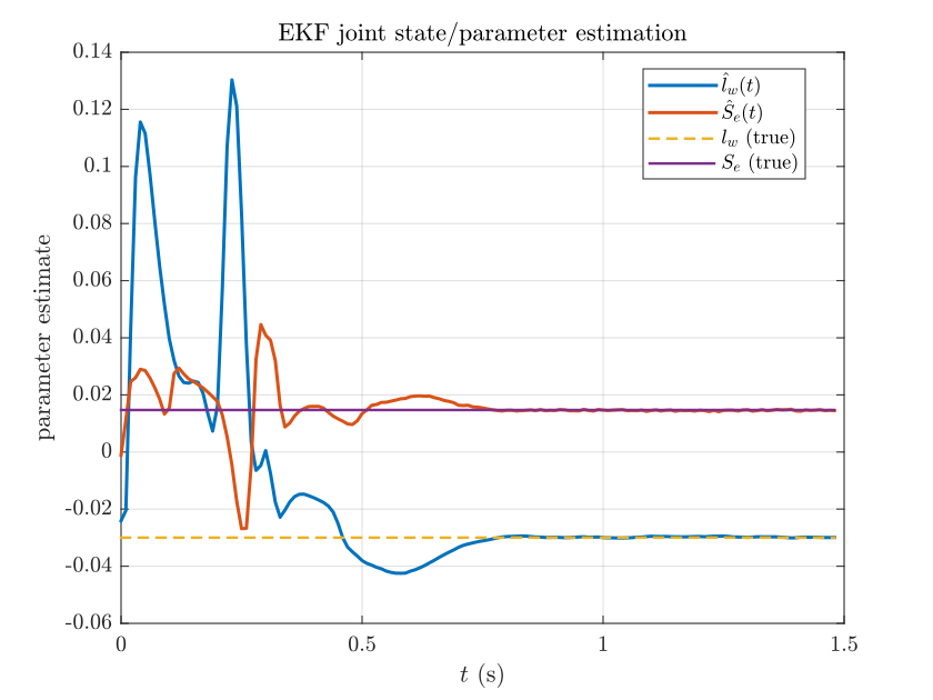
In this demonstration, an infinite-horizon LQR holds the vehicle near cruise while simulated wind drifts, so excitation comes only from disturbance rejection. A perch would be more informative because its large pitch excursion, elevator motion, and post-stall angles make these parameters more observable.

Together, residual learning and parameter estimation provide the data-corrected state-space model used by the planner and controller below.

Planning the maneuver, and protecting it

Forward simulation asks what happens if we replay a chosen input. Trajectory optimization asks the inverse question: does there exist any dynamically consistent motion from the launch state to the perch? Rather than choosing inputs and integrating forward in time order, direct collocation lets the optimizer choose state and input samples together, then constrains the interpolating curve to satisfy the differential equation at collocation points [1].

The notebook does four things, in order:

1. Solve for a nominal trajectory by direct collocation. The launch state is fixed ($x=-3.5$ m, $z=0.1$ m, $\dot x=7$ m/s); the terminal state is pinned to the perch in position with bounded pitch and bounded terminal velocity; elevator angle and elevator rate carry servo limits; there is a running cost on input effort and a terminal quadratic error cost pulling pitch toward $-\pi/4$. Nothing in the problem says pitch up here, stall here, catch the perch here. The timing is discovered.
2. Warm-start a finer mesh from a coarser one. The same program is solved at 25 knot points and then re-solved at 41, seeded by the first solution. The finer problem therefore starts near a feasible maneuver rather than from a fresh interpolated guess.
3. Replay the nominal input open-loop and watch the trajectory drift away from the plan.
4. Wrap the nominal in finite-horizon LQR and re-simulate from several perturbed initial conditions (the launch height is jittered), using the time-varying gain to correct the tracking error $\boldsymbol{x}(t)-\boldsymbol{x}_0(t)$:

The Riccati derivation behind $\boldsymbol{K}(t)$ is standard and lives in [2]. Open-loop replay is the experiment that justifies feedback: dynamics were enforced only at finitely many collocation points, forward integration does not exactly reproduce the transcription, and the maneuver is sensitive. Hardware would add model error on top of that numerical drift.

The division of labor is clean, and it is the reason both pieces are here:

Trajectory optimization finds a feasible schedule for throwing away energy. Finite-horizon LQR defends a neighborhood of that schedule. One answers how should it fly; the other answers if it drifts, can it get back.

The controller is not stabilizing a fixed point but a moving reference, and its authority decays along the way — the maneuver deliberately destroys the dynamic pressure on which control effectiveness depends. In perching that fragility is concentrated near the end, where the terminal geometry is least forgiving.

A note on funnels

A closed-loop rollout is an example: this initial condition worked. The stronger statement is a funnel — a time-varying set $\mathcal{F}(t)$ such that every state inside it at time $t$ is driven to the target set at $t_f$. The usual construction takes the LQR cost-to-go as a Lyapunov candidate, $V(t,\bar{\boldsymbol{x}})=\bar{\boldsymbol{x}}^{\top}\boldsymbol{S}(t)\bar{\boldsymbol{x}}$ with $\bar{\boldsymbol{x}}=\boldsymbol{x}-\boldsymbol{x}_0(t)$, picks a terminal sublevel set inside the acceptable perching set, and integrates backward while requiring the closed-loop vector field to point inward on the boundary. Verifying that condition over a continuum of states is the hard part; sums-of-squares programming with the $S$-procedure turns it into a tractable sufficient certificate. Underactuated develops both the funnel construction and the SOS machinery [1], [3].

The notebook stops at closed-loop simulation from sampled initial conditions. The SOS script in the same directory instead studies the region of attraction of a reversed Van der Pol oscillator, using bilinear alternation between a multiplier step and a $\rho$-maximization step. A perching funnel is therefore a next step rather than a result of this repository; the figure below comes from the experimental work.

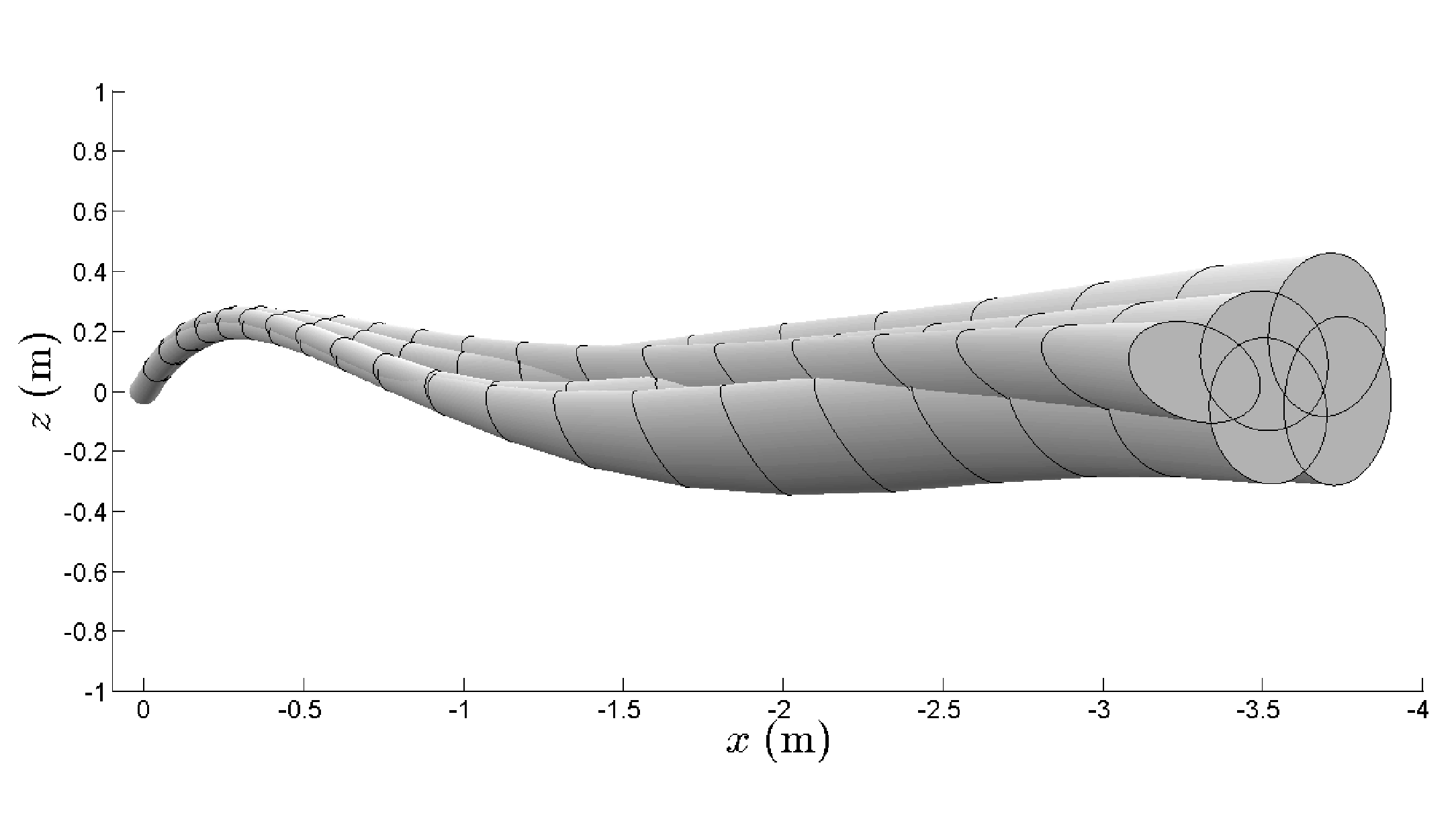
Even when it is not computed, the funnel names the relevant quantity: its width measures how much deviation the closed loop can recover. Shrinking near the perch reflects the loss of control authority in low-speed post-stall flight.

Closing the loop: improving the model the planner uses

So far learning happened before planning. The model-learning script puts it inside the loop: use the current model to plan, execute with local feedback, measure the model error, refit, and plan again.

This is deterministic, structured model-based learning: the controller improves because the point-estimate model it plans through improves. Unlike PILCO, it carries no GP posterior or predictive covariance through the horizon [4].

The planner integrates

where $f_{\mathrm{fp}}$ is the flat-plate model and the columns of $\boldsymbol{G}$ are the RBF features scaled by dynamic pressure and resolved into the lift, drag, and moment directions — so $\boldsymbol{G}\boldsymbol{w}$ is exactly the aerodynamic correction, and the dynamics are affine in the unknowns. The weights start at zero, which means iteration 0 plans through pure flat-plate physics.

Plan. iLQR is used as a fast local optimizer for the current model, returning a nominal maneuver and a time-varying affine policy. Its forward pass rolls out an improved nominal using the feedforward step and a backtracking line search; [1] gives the standard backward pass.

Execute. The feedforward term $\boldsymbol{k}$ is a planning object: the iLQR forward pass uses it to update the nominal control sequence. Execution therefore uses the updated nominal plus local feedback,

with the launch speed randomized each iteration so successive rollouts are not identical.

Identify. Finite differences on the executed rollout give $\dot{\boldsymbol{x}}{\mathrm{data},n}\approx(\boldsymbol{x}{n+1}-\boldsymbol{x}_n)/h$, and because the residual enters affinely, the update is again a ridge least-squares solve — restricted to the three components where the aerodynamic residual acts directly:

Here $\boldsymbol{\Pi}_a$ selects $(\ddot x,\ddot z,\ddot\theta)$; the remaining four equations are kinematic and carry no information about $\boldsymbol{w}$. Rollouts accumulate, so each solve is a batch fit over the full history rather than over the latest flight alone.

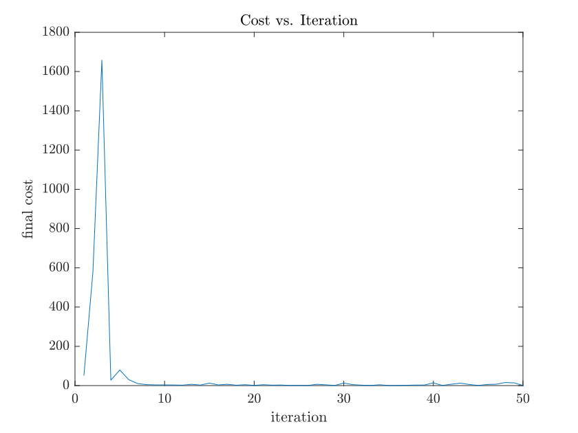
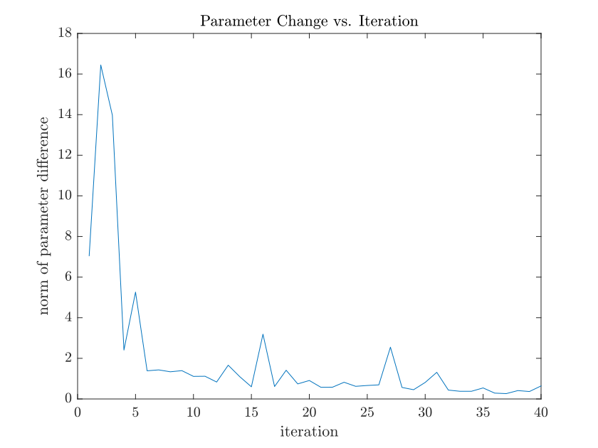
A deliberate mismatch tests the method: the planner’s residual features depend on $(\alpha,\phi)$ — 26 weights per coefficient — while the simulator uses $(\alpha,\phi,V)$ on a finer grid — 126 weights per coefficient. Airspeed dependence is structurally unavailable to the planner. No amount of data can make $\boldsymbol{w}$ represent it.

The loop therefore converges not to the simulator dynamics, but to the best flat-plate-plus-$(\alpha,\phi)$ residual along the states visited by this maneuver. That can be sufficient for replanning. The weight-change plot diagnoses convergence of the fit, while executed terminal cost measures task-relevant improvement.

Two caveats bound the plots: finite differencing amplifies the noise added to measured states, and randomized launch speed makes some terminal-cost variation attributable to the initial condition rather than the model.

Without gradients: CEM and a minimal MPPI-style optimizer

Direct collocation and iLQR exploit derivatives of the dynamics or cost. A separate script includes two sampling-based alternatives that share a rollout function, cost, and horizon.

Both methods optimize one open-loop control sequence $\boldsymbol{U}={u_0,\dots,u_{N-1}}$ over a fixed $0.75$ s horizon and roll candidates through the nonlinear glider model with explicit Euler. The horizon is never shifted and the measured state never triggers replanning, so this is offline sampling-based trajectory optimization, not MPC.

CEM keeps a per-timestep Gaussian over $u_k$ with diagonal variance. Each iteration draws 30 rollouts, keeps the 10 cheapest, and re-estimates the mean and variance by maximum likelihood on that elite set, with a floor on the variance so exploration cannot collapse. It is the cross-entropy idea specialized to a control sequence: refit the sampling distribution to the good samples and repeat.

MPPI keeps a single nominal sequence and perturbs it, $u^{(r)}_k=u_k+\epsilon^{(r)}_k$ with $\epsilon^{(r)}_k$ i.i.d. Gaussian. Rather than a single score per rollout, the implementation forms a time-indexed cost-to-go

turns it into a softmax at each time step,

and moves the nominal by the weighted average of the perturbations,

This is a minimal MPPI-style optimizer. Canonical MPPI adds likelihood-ratio terms to a modified rollout cost and applies the update in a receding-horizon loop; both are absent here [8]. The ME696 notes derive the update from the stochastic HJB equation [4], while [9] gives a KL-regularized interpretation. Numerically, subtracting the minimum cost before exponentiation would preserve the normalized weights while avoiding underflow.

Four details determine how to read the result:

• $\lambda$ controls selection pressure. Small values approach the best sampled rollout; large values approach an unweighted average.
• Perturbation covariance defines the search geometry. It decides whether the samples can reach useful regions of control-sequence space.
• The time-indexed weights are nearly degenerate here. Running cost contains only a small control penalty, while terminal position and pitch dominate. Consequently $S_k^{(r)}$ changes little with $k$ and the update behaves almost like one weight per rollout.
• Search noise is not robustness. The perturbations model neither wind, sensor error, nor aerodynamic uncertainty. Robustness would require sampling those uncertainties or repeatedly replanning from measurements.

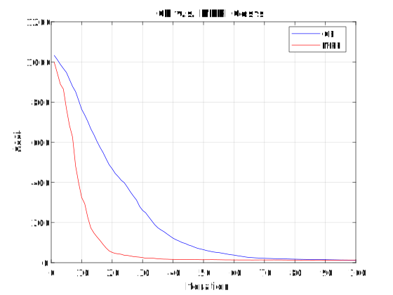
With the same horizon, dynamics, cost, and 30 rollouts per iteration, MPPI descends faster early in this run while CEM improves more evenly and ends at a comparable cost. The methods were not tuned against each other, and their parameters are not commensurate, so this is one observation rather than a ranking.

Across the identification and control pipeline, the useful hierarchy is the same: equation-error fitting can initialize a model, held-out simulation tests whether local errors accumulate, and closed-loop task performance decides whether the model is adequate. Complexity should be added only when the data can identify it and the planner can use it. Perching succeeds because physics, data, optimization, and feedback make the remaining local model error manageable.

References

[1] Russ Tedrake. Underactuated Robotics: Trajectory Optimization. Online course notes. [link]

[2] Russ Tedrake. Underactuated Robotics: Linear Quadratic Regulators — finite-horizon LQR. Online course notes. [link]

[3] Russ Tedrake. Underactuated Robotics: Lyapunov analysis with convex optimization. Online course notes. [link]

[4] Joseph Moore. Learning-Based Control for Robotics. Course notes for JHU ME696, 2025. [link]

[5] Russ Tedrake. Underactuated Robotics: System Identification. Online course notes. [link]

[6] Warren Hoburg and Russ Tedrake. System Identification of Post Stall Aerodynamics for UAV Perching. AIAA Infotech@Aerospace Conference, Seattle, Washington, 2009. [link]

[7] Joseph Moore. Robust Post-Stall Perching with a Fixed-Wing UAV. PhD thesis, Massachusetts Institute of Technology, September 2014. [link]

[8] Grady Williams, Andrew Aldrich, and Evangelos A. Theodorou. Model Predictive Path Integral Control: From Theory to Parallel Computation. Journal of Guidance, Control, and Dynamics, 40(2):344–357, 2017. [link]

[9] Heng Yang. Optimal Control and Reinforcement Learning, Ch. 4: Model-Based Planning and Optimization. Textbook for Harvard ES/AM 158, 2025. [link]