Mehrotra’s Predictor–Corrector Interior-Point Method
How affine prediction, adaptive centering, and a second-order correction turn the KKT equations of a convex QP into a practical solver.
For a compact executable version of the QP equations below, see barrierQP.
A quadratic program has a quadratic objective and linear constraints, so one might expect Newton’s method to solve it in a single step. That is almost true. After introducing slack variables, stationarity and primal feasibility are affine equations. The only nonlinear KKT equation is complementarity, \(s_i z_i=0\), and nearly all of the interesting interior-point machinery is organized around that one product.
Mehrotra’s predictor–corrector method handles it in an unusually economical way. At each iterate it first asks where an aggressive affine-scaling step would go if complementarity were driven directly to zero. That hypothetical step is not accepted. Instead, it is used twice: to choose how strongly the next direction should be centered, and to estimate the second-order term discarded by the Newton model. A second solve then corrects the model. Both solves use the same KKT matrix, so the expensive factorization is reused.
This is the main idea of the method. The rest of the article makes each part of that statement precise.
Mehrotra’s 1992 paper develops the method for linear programs. The presentation below uses the now-standard convex QP form found in CVXOPT, CVXGEN, and HPIPM. The Hessian changes the linear algebra, but the predictor–corrector mechanism still lives in complementarity.
KKT Conditions for a Convex QP
Consider the convex quadratic program
Introduce a slack \(s\in\mathbb R^m\) and dual variables \(y\) and \(z\):
\[Gx+s=h, \qquad s\ge0,\quad z\ge0.\]The KKT residuals are
and optimality additionally requires
where \(\odot\) denotes elementwise multiplication. The first three equations are affine in the primal–dual variables. Equation (3) is the only nonlinear one.
An interior-point method avoids the boundary by keeping \(s,z\succ0\) and replacing (3) with
For feasible points, these equations describe the central path. The parameter
\[\mu=\frac{s^\top z}{m}\]is the average complementarity, and \(s^\top z=m\mu\) is the surrogate duality gap. As \(\mu\) decreases, the path approaches a KKT point. Componentwise centrality matters: a small average can still hide a few badly unbalanced pairs \(s_i z_i\). This is the primal–dual version of the central-path picture developed in Chapter 11 of Convex Optimization.
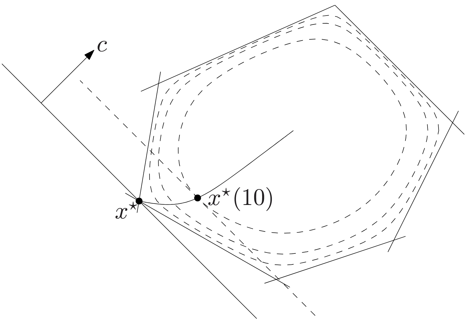
The iterates of an infeasible-start method need not lie exactly on this path, or even satisfy the linear constraints. The path is a geometric guide; the algorithm works with all four residual blocks at once.
The Primal–Dual Newton System
Let \(S=\operatorname{diag}(s)\), \(Z=\operatorname{diag}(z)\), and stack the variables as \(w=(x,y,z,s)\). Linearizing the KKT equations around the current iterate gives the Jacobian
\[J= \begin{bmatrix} P & A^\top & G^\top & 0\\ A & 0 & 0 & 0\\ G & 0 & 0 & I\\ 0 & 0 & S & Z \end{bmatrix}.\]A primal–dual Newton direction toward a complementarity target \(\mu_t\) solves
Notice what does not appear in \(J\): the target \(\mu_t\). At a fixed iterate, changing the desired complementarity changes only the right-hand side. This is the computational opening exploited by the predictor–corrector method.
There is also a useful central-path interpretation. If \(w^\star(\mu)\) is exactly on the path, implicit differentiation of the perturbed KKT equations gives
\[J\frac{dw^\star}{d\mu} = \begin{bmatrix}0\\0\\0\\\mathbf 1\end{bmatrix}.\]A first-order prediction from the current \(\mu\) toward \(0\) therefore satisfies
Thus, on the central path, the affine-scaling direction is exactly the tangent prediction obtained by aiming at zero complementarity. Away from the path this is only the geometric intuition: the actual direction must also reduce \(r_d,r_e,r_i\). In Mehrotra’s original formulation, the broader interpretation is a local expansion of a primal–dual affine-scaling trajectory from the current positive point.
The Affine-Scaling Predictor
The predictor chooses the most aggressive possible target, \(\mu_t=0\):
If the linear model were exact and a full step remained interior, this direction would satisfy the unperturbed KKT equations in one move. Usually it heads toward the boundary. We compute the largest hypothetical step that preserves nonnegativity,
and inspect the complementarity at that affine point:
The important word is inspect. The affine point is a prediction, not the next iterate. Its job is to report how much progress the current Newton geometry appears to permit.
That report determines the centering parameter. A standard QP implementation uses
If the affine probe predicts a large reduction in complementarity, then \(\mu_{\mathrm{aff}}/\mu\) is small and so is \(\sigma\): the combined direction can remain aggressive. If the probe makes little progress, \(\sigma\) grows and pulls more strongly toward the center. The cube is a successful heuristic rather than a consequence of Newton’s method; variants of the exponent and clipping rule appear in different implementations.
This feedback is one of Mehrotra’s most useful ideas. Instead of prescribing a barrier schedule in advance, the method asks the current linearized problem how ambitious the next target should be.
The Centering-Corrector Direction
Centering alone is not the whole second solve. The exact complementarity after a step is
Newton’s method retains the two linear terms and discards the product of the directions. For the affine predictor,
\[Z\Delta s^{\mathrm{aff}} +S\Delta z^{\mathrm{aff}} =-s\odot z,\]so the complementarity left by a full affine step is precisely the omitted quadratic term
\[\Delta s^{\mathrm{aff}}\odot\Delta z^{\mathrm{aff}}.\]The predictor has therefore done more than estimate a step length. It has measured the leading error of its own linear model. Mehrotra’s corrector uses that measurement while also adding the adaptive centering target:
The two terms in the last block play different roles. The centering term \(\sigma\mu\mathbf 1\) prevents a few complementarity pairs from collapsing much faster than the others. The correction term subtracts a concrete second-order defect revealed by the affine solve.
This also clarifies a common misconception about the name predictor–corrector. It does not mean that the solver accepts an affine update and then repairs the new point. Both directions are computed at the same current iterate. Equivalently, the combined direction solves (5) with complementarity right-hand side
\[-s\odot z +\sigma\mu\mathbf 1 -\Delta s^{\mathrm{aff}}\odot\Delta z^{\mathrm{aff}}.\]The correction is called second-order because it restores information from the product in (11), even though it is obtained through another linear solve.
The Reduced KKT System
The four-by-four system in (5) explains the algorithm, but a QP solver will usually eliminate \(\Delta s\) and \(\Delta z\) before factorization. For a generic right-hand side
\[J\Delta w=(b_d,b_e,b_i,b_c),\]define \(D=S^{-1}Z=\operatorname{diag}(z/s)\). Block elimination gives
The remaining directions follow from
\[\Delta s=b_i-G\Delta x, \qquad \Delta z=S^{-1}(b_c-Z\Delta s).\]This reduced saddle-point matrix is the numerical core of many second-order QP solvers. At one iterate, \(D\) is fixed. The affine and corrector systems change \(b_c\), not the matrix in (13), so the solver can factor the matrix once and apply the factors to two right-hand sides. The second direction is not free, but triangular back-solves are usually much cheaper than another sparse factorization.
Operationally, an iteration is now quite short: evaluate the residuals, form and factor (13), solve for the affine direction, compute \(\mu_{\mathrm{aff}}\), \(\sigma\), and the quadratic defect, solve the corrected right-hand side with the stored factors, and choose a safe step. That sequence is most of the algorithm.
The same equation also exposes a central numerical difficulty. Near a strictly complementary solution, an active constraint tends to have \(s_i\to0\) and \(z_i>0\), while an inactive one has \(z_i\to0\) and \(s_i>0\). The diagonal ratios \(z_i/s_i\) can therefore span many orders of magnitude. The mathematical path approaches the solution just as its linear algebra becomes increasingly ill-conditioned.
This is where a compact derivation stops and a production solver begins. CVXGEN combines static and dynamic regularization with iterative refinement; HPIPM adds residual checks, regularization, refinement, and structure-specific factorizations. For optimal-control QPs, the same saddle-point solve can be organized as a Riccati recursion rather than a generic sparse \(LDL^\top\) factorization. These choices change the numerical machinery, not the predictor–corrector logic.
Step Size and Termination
After combining the directions, choose the largest step that stays inside the orthant,
\[\alpha_{\max} =\sup\left\{ \alpha\ge0 \;\middle|\; s+\alpha\Delta s\ge0, \ z+\alpha\Delta z\ge0 \right\},\]and take a fraction-to-the-boundary step
Some implementations use separate primal and dual step lengths; the common-step form keeps the notation compact. In either case, the affine boundary step in (8) is used to make a prediction, whereas (14) updates the actual iterate.
Positivity alone is not a stopping condition. An infeasible-start method must separately verify primal feasibility, stationarity, and complementarity, for example
A tiny gap does not imply a solved KKT system. Conversely, small primal and dual residuals do not imply complementarity. Practical solvers scale these tests relative to the problem data and add safeguards for small steps, non-finite directions, or insufficient progress.
Initialization
An infeasible-start method does not need a feasible initial point, but it does need \(s^0,z^0\succ0\). One useful QP initialization, used in the CVXOPT cone-program notes and in CVXGEN, begins with the regularized system
The second block gives provisional slacks \(\widetilde s=h-Gx^0=-\widetilde z\). Shift the primal and dual quantities independently,
\[s^0=\widetilde s+\delta_p\mathbf 1, \qquad z^0=\widetilde z+\delta_d\mathbf 1,\]using the smallest nonnegative shifts, with a modest margin, that make both vectors strictly positive. The shifts generally destroy exact primal or dual feasibility, which is acceptable: the residuals in (2) are already part of the Newton system.
This initialization is not part of the essential Mehrotra correction, nor is it meant to guess the optimizer. It simply creates a symmetric, numerically moderate point from which the infeasible-start iteration can begin. Different solvers use different starting strategies.
Extension to Conic Constraints
Ordinary QP inequalities are already conic constraints over the nonnegative orthant. Replacing that orthant by a second-order or positive-semidefinite cone changes the geometry of complementarity, but not the overall organization of the method.
For a cone \(K\), a logarithmically homogeneous barrier \(f\), a primal slack \(s\in K\), and a dual variable \(z\in K^\ast\), centrality can be written as
For symmetric cones—nonnegative orthants, second-order cones, and positive-semidefinite cones—this becomes
where \(\circ\) is the cone’s Jordan product and \(e\) its identity. The orthant recovers elementwise multiplication. A second-order cone instead couples a whole vector block, so componentwise positivity becomes cone interiority and the diagonal scaling in (13) becomes a cone-scaling block.
The corrector survives, but it must be written in the right coordinates. With Nesterov–Todd scaling \(W\), the symmetric-cone analogue of the quadratic defect has the form
\[\eta = \bigl(W^{-1}\Delta s^{\mathrm{aff}}\bigr) \circ \bigl(W\Delta z^{\mathrm{aff}}\bigr).\]For nonsymmetric cones such as exponential and power cones, there is no Jordan algebra and this formula does not apply; solvers such as Clarabel use barrier derivatives and a different higher-order correction. The durable idea is not a particular elementwise product. It is to use an aggressive affine solve to estimate both the attainable progress and the nonlinear defect, then reuse the same local KKT geometry for a corrected direction.
Summary
Under the hood, a second-order QP solver is not repeatedly solving a new optimization problem from scratch. It maintains an interior primal–dual state, forms one local KKT geometry, probes that geometry with a target of zero complementarity, lets the probe choose the centering strength, corrects the nonlinear term that the local model omitted, and then takes the largest safe step. Most of the time is spent factoring a structured indefinite matrix; much of solver design is about making that factorization reliable as the central path becomes ill-conditioned.
That is why Mehrotra’s method is more than “two Newton steps.” The first solve is an experiment. The second uses what the experiment revealed while the expensive linear algebra is still available. This predictor–corrector pattern appears, with different scaling and safeguards, in QP solvers such as CVXGEN, qpSWIFT, and HPIPM, and continues into modern conic solvers.
For a compact executable version of the QP equations above, see barrierQP.
References
-
S. Mehrotra, On the Implementation of a Primal-Dual Interior Point Method, SIAM Journal on Optimization, 2(4):575–601, 1992.
-
S. Boyd and L. Vandenberghe, Convex Optimization, Chapter 11, Cambridge University Press, 2004.
-
L. Vandenberghe, The CVXOPT Linear and Quadratic Cone Program Solvers, 2010.
-
J. Mattingley and S. Boyd, CVXGEN: A Code Generator for Embedded Convex Optimization, Optimization and Engineering, 13(1):1–27, 2012.
-
G. Frison and M. Diehl, HPIPM: A High-Performance Quadratic Programming Framework for Model Predictive Control, arXiv:2003.02547, 2020.
-
A. G. Pandala, Y. Ding, and H.-W. Park, qpSWIFT: A Real-Time Sparse Quadratic Program Solver for Robotic Applications, IEEE Robotics and Automation Letters, 4(4):3355–3362, 2019.
-
P. J. Goulart and Y. Chen, Clarabel: An Interior-Point Solver for Conic Programs with Quadratic Objectives, arXiv:2405.12762, 2024.