Convexification in Trajectory Optimization
How lossless convexification, successive convexification, and continuous-time path-constraint formulations expose and reuse convex structure in trajectory optimization.
The complete code for this post is in Convexification.
Convexification is often described as a solver strategy, but in trajectory optimization it can make three mathematically different promises. A relaxation may reveal that a structured nonconvex problem was convex in disguise. A sequence of local models may recover useful convexity after nonlinear dynamics destroy that structure. Or the continuous problem may be reformulated so that a finite transcription records information that isolated nodes omit. These promises answer different questions: whether one convex solve recovers the original optimum, whether repeated convex solves approach a stationary trajectory, and whether the computed trajectory represents a continuous-time path claim.
Consider a path-constrained optimal-control problem:
\[\begin{aligned} \min_{x(\cdot),u(\cdot),t_f}\quad & \Phi(x(t_f),t_f)+\int_0^{t_f}L(x(t),u(t))\,dt,\\ \text{s.t.}\quad & \dot x(t)=f(x(t),u(t)),\\ & g(x(t),u(t))\le 0,\qquad h(x(t),u(t))=0,\\ & x(0)=x_{\mathrm{init}},\qquad \psi(x(t_f),t_f)=0. \end{aligned}\]Several difficulties are compressed into this notation. The dynamics may be nonlinear, the control set nonconvex, the final time unknown, and state or obstacle constraints curved. Discretization adds a different issue: satisfying a constraint at finitely many nodes is not the same statement as satisfying it at every time.
Convexity is therefore not merely a choice of solver. It describes what remains of the original problem after a change of variables, a relaxation, or a local approximation. In the line of work considered here, that meaning changes three times:
-
Lossless convexification (LCvx) exposes a convex formulation hidden inside a specially structured nonconvex problem.
-
Successive convexification (SCvx) constructs a new local convex model at every outer iteration when no globally exact one-shot formulation is available.
-
Continuous-Time SCvx (CT-SCvx) first changes how path constraints are represented, then applies a prox-linear method to the resulting finite-dimensional problem.
LCvx is the conceptual and historical beginning of this research line, rather than a mathematical prerequisite for SCvx. The common subject is convexification; the object being convexified, and therefore the conclusion one may draw, changes at each stage. The development below follows that change by asking the same four questions each time: what failed, what changed mathematically, what did the change buy, and what limitation remained?
Lossless convexification (LCvx)
Lower thrust-magnitude bound
The landing example in Açıkmeşe and Blackmore’s 2011 paper [1] contains a lower and upper bound on thrust magnitude. Introducing an auxiliary magnitude $\sigma(t)$ gives
\[\begin{aligned} \text{original:}\quad& \rho_{\min}\le \lVert T(t)\rVert_2\le \rho_{\max},\\ \text{relaxed:}\quad& \lVert T(t)\rVert_2\le \sigma(t),\qquad \rho_{\min}\le \sigma(t)\le\rho_{\max},\\ \text{tight optimum:}\quad& \lVert T^\star(t)\rVert_2=\sigma^\star(t)\quad\text{a.e.} \end{aligned}\]The upper bound describes a Euclidean ball. The positive lower bound removes its center, producing an annulus in two dimensions and a spherical shell in three. Two admissible thrust vectors on opposite sides can have an inadmissible average, so the original set is nonconvex.
The lifted inequalities are convex and second-order-cone representable. They are also a relaxation: they allow $\lVert T\rVert_2<\rho_{\min}$ while $\sigma\ge\rho_{\min}$. Lifting makes the problem easier by adding freedom; it does not, by itself, show that the relaxed optimum solves the original problem.
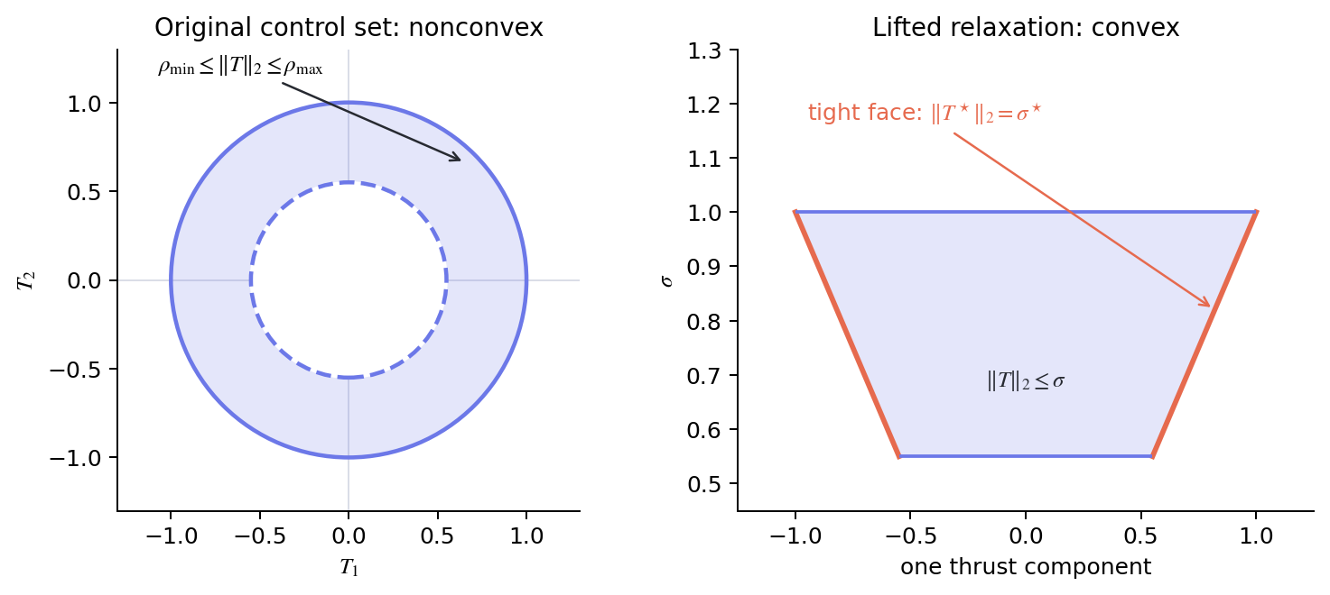
The essential result is the equality in the last line. Under the controllability, terminal-transversality, and strict state-interiority conditions stated in the paper, the relaxed problem admits an optimal control satisfying the original nonconvex magnitude constraint almost everywhere. The proof uses the Pontryagin Minimum Principle: the costate and switching structure determine the optimal control direction, and a persistent positive gap $\sigma-\lVert T\rVert_2$ conflicts with the necessary optimality conditions under the paper’s nondegeneracy assumptions.
The transferable insight is shorter than the proof:
The computational move is lifting. The mathematical move is proving that the added freedom is not useful at an optimum.
Within that structured model, a globally solved convex problem recovers a global solution of the original nonconvex control problem under the theorem’s assumptions. Here “global” belongs to the specified model and its convex transcription. It says nothing about physical effects omitted from the model, numerical integration error, or finite solver tolerances.
Powered-descent formulation
The 2013 soft-landing paper [2] turns this theorem into a complete formulation. For position $r$, velocity $v$, mass $m$, and commanded thrust $T_c$, define log mass, mass-normalized thrust, and its lifted magnitude by
\[\begin{aligned} z&=\log m,& u&=\frac{T_c}{m},& \sigma&=\frac{\Gamma}{m},\\ \dot r&=v,& \dot v&=g+u,& \dot z&=-\alpha\sigma,\\ \lVert u\rVert_2&\le\sigma,& \hat e^\top u&\ge\sigma\cos\theta_{\max}.& \end{aligned}\]The first cone is the relaxed thrust-magnitude relation. The second is the thrust-pointing constraint. Boundary conditions prescribe the initial state and desired terminal position and velocity; speed and glide-slope bounds are convex state constraints; maximizing terminal log mass is equivalent to maximizing final mass. For fixed final time, these pieces form an SOCP-compatible point-mass landing problem.
The actual paper writes translation in a planet-fixed rotating frame. Coriolis and centrifugal terms therefore appear in its state matrix, but the dynamics remain affine in state and mass-normalized thrust. Suppressing those terms in the display above exposes the conic structure without changing the convexity argument.
The model also separates the landing objective into two convex problems. Problem 3 first minimizes horizontal terminal miss distance while enforcing touchdown altitude and zero terminal velocity. Problem 4 then minimizes fuel subject to achieving no worse than that optimal miss distance. This lexicographic construction prevents fuel economy from being purchased by accepting an avoidable landing error.
The resulting program is complete in the formulation sense: initial and terminal conditions, mass depletion, velocity, glide slope, thrust magnitude, and pointing all appear in one consistent optimization model. For a prescribed time of flight, the solve is convex. When final time is selected outside that formulation, evaluating a bounded set or one-dimensional family of candidate times still differs fundamentally from iterating local models of the entire trajectory.
Two operations in this formulation should not be conflated. The relaxation of the lower thrust bound is the object of the losslessness theorem. After $z=\log m$, the mass-dependent normalized-thrust bounds still contain exponentials; the 2013 construction replaces them with conservative convex approximations about prescribed mass profiles. The former is proved tight under structural assumptions. The latter is an approximation whose conservatism remains part of the finite model.
This is a formulation breakthrough rather than an iterative nonlinear algorithm. It works because the dynamics, objective, boundary conditions, and control geometry have been selected so that one convex program—or a small outer family when a scalar parameter such as final time is searched—retains the relevant optimum.
That architecture has a boundary. Once attitude kinematics, angular velocity, torque, gimbal geometry, and other nonlinear effects enter the state dynamics, the entire problem no longer shares the same one-shot hidden convexity. The next step is not a stronger claim of losslessness, but a different use of convex structure.
Successive convexification (SCvx)
For general nonlinear dynamics $\dot x=f(x,u)$, SCvx begins with a reference trajectory $(\bar x^j,\bar u^j)$ and a first-order model
\[\begin{aligned} \dot x &\approx f(\bar x^j,\bar u^j) +A^j(t)(x-\bar x^j) +B^j(t)(u-\bar u^j),\\ A^j(t)&=\frac{\partial f}{\partial x}(\bar x^j,\bar u^j),\\ B^j(t)&=\frac{\partial f}{\partial u}(\bar x^j,\bar u^j). \end{aligned}\]The affine model can enter a convex subproblem, but linearization creates two new failure modes. The first is artificial infeasibility: approximate dynamics and hard boundary conditions may be mutually inconsistent even when the nonlinear problem is feasible. Mao, Szmuk, and Açıkmeşe [3] add a heavily penalized virtual control $v$:
\[\dot x=A^j x+B^j u+c^j+E^jv, \qquad J_{\mathrm{vc}}=w_v\int_0^{t_f}\lVert v(t)\rVert_1\,dt.\]Virtual control is a feasibility device rather than a physical actuator. It lets an early convex subproblem be solved from a dynamically inconsistent reference. Its norm must become negligible before the trajectory can be interpreted as a solution of the physical dynamics.
The second failure is an untrustworthy step. Far from the reference, a first-order model may expose false descent directions—artificial unboundedness in the paper—or merely predict an improvement that the nonlinear problem does not realize. The 2016 algorithm bounds the step and asks the nonlinear penalized objective to judge the convex prediction:
\[\lVert z-\bar z^j\rVert\le\Delta_j, \qquad \varrho_j= \frac{J_{\mathrm{nl}}(\bar z^j)-J_{\mathrm{nl}}(z^{j+1})} {J_{\mathrm{nl}}(\bar z^j)-J_{\mathrm{cvx}}^j(z^{j+1})}.\]A poor ratio rejects the candidate and contracts $\Delta_j$; a good ratio accepts it and may enlarge the next region. The mechanism can be read as a short loop:
reference trajectory
→ local affine model with virtual control
→ convex subproblem inside a trust region
→ nonlinear model-agreement test
→ accept or reject, then update the radius
Repeated convexification is therefore different from repeated relaxation in the LCvx sense. LCvx proves that one enlarged feasible set is tight for a structured problem. SCvx leaves the general problem nonconvex and asks each convex model only for a locally useful step.
The 2016 algorithmic exposition assumes that state and control constraints are already convex or have been convexified separately; nonlinear dynamics are the principal object linearized successively. Its convergence analysis is posed in continuous function spaces, independent of one particular numerical transcription.
A software implementation must nevertheless parameterize controls and discretize or integrate the local dynamics. The accuracy of that finite representation remains a separate question.
This also explains why SCvx can start from a trajectory that does not satisfy the dynamics. Virtual control prevents an early dead end, while the trust mechanism limits the effect of an inaccurate model.
The result remains local: the reference influences the basin reached, and a stationary point of a generic nonlinear OCP need not be globally optimal. The cart-pole experiment later makes this separation visible, first through the failure of one affine model and then through repeated repair of nonlinear dynamic agreement.
An algorithmic skeleton is not yet a flight solver. Time, controls, sensitivities, scaling, and nonlinear validation must all be specified before the loop becomes an implementation.
SCvx for free-final-time 6-DoF powered descent
The 2018 free-final-time Mars landing paper [4] supplies that architecture. Its state contains position, velocity, a scalar-first attitude quaternion, angular velocity, and mass. A gimbaled engine produces force and torque, while final time is itself optimized. The transferable contribution is less the list of rigid-body equations than the route from those equations to a sequence of scaled SOCPs.
The state already shows why the point-mass construction no longer closes in one step. Quaternion kinematics couple attitude and angular velocity; rotational acceleration contains $\omega\times J\omega$; attitude rotates body-frame thrust into the inertial frame; and normalized dynamics couple every state equation to final time.
Upper thrust, gimbal angle, glide slope, and angular-rate bounds retain convex forms. The remaining nonlinear expressions are linearized about the current trajectory, so the solver preserves exact convex pieces and approximates only the obstruction to the next convex subproblem.
Physical time $t\in[0,t_f]$ is mapped to normalized time $\tau\in[0,1]$. The final time becomes a dilation variable coupled to the dynamics. With first-order-hold (FOH) control, continuous-time linearization and interval integration give a discrete local model of the form
\[\begin{aligned} \frac{dx}{d\tau}&=t_f f(x(\tau),u(\tau)),\\ u(\tau)&=\lambda_k^-(\tau)u_k+\lambda_k^+(\tau)u_{k+1},\\ x_{k+1}&=A_kx_k+B_k^-u_k+B_k^+u_{k+1}+S_k t_f+c_k+\nu_k. \end{aligned}\]The matrices are obtained by more than freezing the dynamics for an Euler step. Along each reference segment, the state-transition matrix is integrated together with sensitivities to the left and right FOH controls and to final time. The resulting map carries the continuous-time linearized model across the interval.
This is the source of the phrase “exact discretization” in the paper. Its scope is narrow: the discrete relation above is the exact interval map of the linear time-varying local model if the associated matrix differential equations are integrated exactly. The nonlinear dynamics have still been linearized, and software evaluates the state and sensitivity equations to finite numerical tolerance.
One outer iteration can be summarized without a separate solver diagram:
reference trajectory
→ propagate the nonlinear reference and integrate sensitivities
→ assemble and scale one SOCP
→ solve for a candidate trajectory
→ update the reference and repeat
Nondimensionalization keeps quaternion components, angular rates, positions, thrust, mass, and time on comparable numerical scales. Virtual control relaxes the discrete dynamics, while a penalized trust term discourages large changes from the reference. This 2018 implementation uses a soft trust treatment and tests virtual control and iterate changes at termination. That is a distinct algorithmic choice from the ratio-managed hard trust region in the 2016 presentation.
Initialization shows how the pieces cooperate. The paper begins from simple state and thrust profiles that need not satisfy the nonlinear rigid-body equations. The first propagation records their local sensitivities, virtual control makes the boundary-value subproblem solvable, and the trust penalty keeps the candidate near information supplied by the reference.
Each accepted trajectory then supplies the next nominal flow and interval matrices. Dynamic consistency is recovered through the repeated linearize–integrate–solve cycle instead of being required at initialization.
The paper thereby turns the abstract SCvx loop into a complete free-final-time 6-DoF solver: initialize a reference, propagate and linearize continuously, integrate interval sensitivities, solve a scaled cone program, update the reference, and check nonlinear dynamic consistency. Its examples demonstrate that architecture for the stated vehicle and numerical setup.
The paper also says that this variant is similar, but not identical, to the 2016 SCvx algorithm and does not inherit that convergence proof directly. Its reported timings characterize those implementations rather than every powered-descent problem.
Convergence results and qualifications
Numerical success and a theorem about the generated sequence answer different questions. The 2018/2019 convergence paper [5] studies a finite-dimensional SCvx formulation after nonlinear equalities and inequalities have been placed in an $\ell_1$ exact-penalty objective. Schematically:
\[\min_{z\in\mathcal Z} J_0(z) +\lambda\lVert F(z)\rVert_1 +\lambda\lVert[g(z)]_+\rVert_1.\]Here $\mathcal Z$ contains the remaining convex constraints. Exact penalization connects first-order properties of the nonsmooth penalized problem to those of the constrained problem at a finite penalty weight. Feasibility, a sufficiently large $\lambda$, and the relevant constraint qualifications are what allow a stationary point or local minimizer to recover the corresponding KKT or local-optimality statement. The penalty alone supplies neither feasibility nor global optimality.
Three levels of convergence must then be separated. Weak convergence concerns stationary accumulation points. Strong convergence means that the whole sequence approaches one limit. A superlinear rate is a still more local statement about how quickly iterates approach that limit.
The original paper claimed all three, using a Kurdyka–Łojasiewicz argument for whole-sequence convergence and structural optimal-control assumptions for the local rate. Its word “global” described the reach of the convergence analysis from arbitrary initialization, not convergence to a global minimizer.
The 2024 Remarks paper [6] identifies where this chain overreached. The exact-penalty theorem cited in the first direction of the original Theorem 3.9 requires a local minimizer, rather than merely a KKT point. Bounded iterates require a compact level-set assumption.
More seriously, Eq. (3.33) does not follow from the lemmas used in the KL proof, so Section 3.2 does not establish strong convergence under its original assumptions. The superlinear proof also needs the entire sequence to converge to the same point; convergence of one subsequence is insufficient.
The note reconnects SCvx to trust-region results of Zhang from 1985 and 1989. With compact level sets, the stationary-accumulation-point result remains the baseline conclusion. Strong convergence and the superlinear rate can be recovered near a feasible limit under tighter local growth conditions inherited from LICQ, strict complementarity, and a sufficient set of binding constraints.
These conditions are appreciably stronger than a generic claim of “SCvx is superlinear.”
The correction changes the proof and the scope of its conclusions, not the iteration or the reported numerical trajectories. The careful statement is therefore: SCvx has stationary accumulation-point guarantees for the penalized finite problem under compactness and regularity assumptions; feasible stationary points can recover first-order conditions of the constrained problem with a sufficiently large penalty; whole-sequence and superlinear conclusions require stronger local hypotheses.
Even perfect convergence of a node-constrained problem leaves another logical gap untouched.
Continuous-time path-constraint representation
Suppose virtual control is negligible, shooting defects are small, and every grid node satisfies a path inequality. The implication
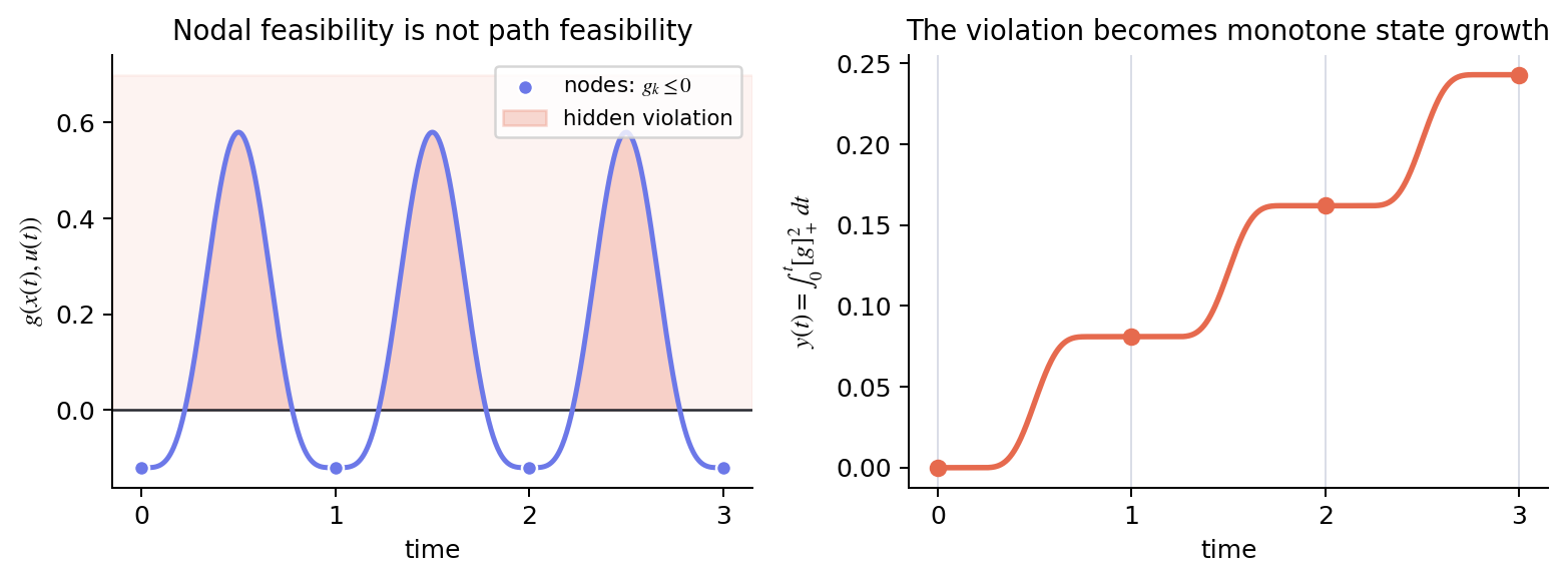
\[g(x_k,u_k)\le0 \quad\not\Rightarrow\quad g(x(t),u(t))\le0 \quad\forall t\in[t_k,t_{k+1}]\]is false. A rocket can cross a glide-slope cone between knots, an interpolated path can enter an obstacle, or a cart can leave its finite track and return before the next node. A finer grid may reduce the observed error, but it still asserts only a larger finite collection of inequalities.
Accumulated violation state
Elango et al. [7] instead put the missing inter-sample information into the dynamics before discretization. For inequalities $g_i(x,u)\le0$ and equalities $h_j(x,u)=0$, one admissible nonnegative exterior measure is
\[\begin{aligned} \Lambda(x,u) &=\sum_i[g_i(x,u)]_+^2+\sum_j h_j(x,u)^2, \qquad [a]_+=\max(a,0),\\ \dot y(t)&=\Lambda(x(t),u(t)),\qquad y(0)=0. \end{aligned}\]The paper permits a broader class of exterior penalties; the squared positive-part and squared equality residual make the logic immediate. Because $\Lambda\ge0$, $y$ is nondecreasing. Lemma 2 and Corollary 3 show that $y(t_f)=0$ is equivalent to path feasibility almost everywhere along the corresponding trajectory.
If the composed path functions are continuous on an interval, any positive violation persists on a neighborhood and contributes positive area. Zero accumulation then gives pointwise feasibility on that segment.
The change is representational: a path predicate has become an endpoint condition on a monotone state. Multiple shooting will later sample $y$ at interval boundaries, but each increment already contains an integral over the whole interval.
Relaxation of the zero-accumulation condition
Exact zero accumulation creates a constraint-qualification problem. At a feasible point, the gradient of the squared exterior penalty vanishes. Combining the accumulated-state shooting equation with a zero-increment boundary condition then makes active constraint gradients structurally dependent, violating LICQ. The paper uses the positive interval relaxation
\[y_{k+1}-y_k\le\varepsilon, \qquad \varepsilon>0.\]The relaxation also has a quantitative interpretation. Under the compact control and dilation sets, bounded path-derivative, and minimum interval-length assumptions of Theorem 14, a scalar path component with derivative bound $\omega$ satisfies
\[\max_{t\in[t_k,t_{k+1}]}[g(t)]_+ \le (4\varepsilon\omega)^{1/3}\]when $\varepsilon\le\omega^2\Delta t_{\min}^3/4$. An analogous absolute-value bound holds for equality constraints. Thus zero accumulation gives the exact almost-everywhere statement, whereas positive $\varepsilon$ gives a conditional violation bound. In computation, the usefulness of that bound depends on defensible derivative constants; dense rollout remains a separate numerical check on the returned trajectory.
Finite-dimensional multiple shooting
The reformulated OCP is made finite-dimensional through control parameterization, generalized time dilation, and multiple shooting. Let $s(\tau)>0$ satisfy $dt/d\tau=s(\tau)$, and collect the physical state, accumulated violation, physical time, and any running-cost state into $\xi$. Over interval $k$,
\[\xi_{k+1}=\Phi_k(\xi_k,q_k), \qquad d_k=\xi_{k+1}-\Phi_k(\xi_k,q_k),\]where $q_k$ contains the interval control and dilation parameters. The nodal values $\xi_k$ are independent shooting variables, and the nonlinear residuals $d_k$ enforce agreement with the interval flow. That flow carries physical dynamics, running cost, elapsed time, and accumulated violation together. Its first derivatives follow from variational differential equations.
Generalized dilation is richer than one scalar final time: the positive function $s(\tau)$ distributes physical duration across intervals. The physical clock satisfies $t’=s$, and the state, running-cost, and violation dynamics receive the same factor. The fixed-final-time notebook experiments do not exercise this layer, but it is part of the general formulation.
As a mathematical object, $\Phi_k$ is the exact solution operator of an initial-value problem. Code approximates it and its sensitivities with a numerical integrator. Reporting both shooting defects and an independently evaluated dense nonlinear rollout keeps that numerical approximation visible.
Convex-composite and prox-linear formulation
After parameterization and multiple shooting, smooth nonlinear flow and boundary residuals are collected in $G(z)$. A convex outer function $H$ contains the terminal cost and $\ell_1$ exact penalties, while $J(z)=\delta_{\mathcal Z}(z)$ retains the directly representable convex constraints. This gives the convex-composite objective and its prox-linear model:
\[\begin{aligned} \Theta_\gamma(z)&=J(z)+H(G(z)),\\ z^{j+1}\in\arg\min_{z\in\mathcal Z}\quad& H\!\left(G(z^j)+DG(z^j)(z-z^j)\right) +\frac{1}{2\rho_j}\lVert z-z^j\rVert_2^2. \end{aligned}\]Here $\gamma$ is the exact-penalty weight and $\rho_j$ sets the proximal step scale. Each layer has one role: $G$ preserves nonlinear flow information, $H$ preserves convex nonsmooth structure, $DG(z^j)$ supplies the local model, and the proximal term controls its locality. The last term plays a trust-like role, but the subproblem and analysis now come from convex-composite minimization rather than the hard-radius presentation of 2016.
CT-SCvx is therefore more than SCvx with one extra state. It changes the OCP representation, the finite multiple-shooting problem, and the optimization framework applied to that problem.
Under the paper’s smoothness, boundedness, and proximal-step assumptions, prox-linear iterations approach stationarity of the penalized finite problem. A stationary point that is feasible for the control-parameterized multiple-shooting problem is a KKT point under the stated regularity conditions; conversely, a KKT point is stationary for a sufficiently large finite penalty. For the convex OCP specialization, strong Slater and the penalty/proximal conditions strengthen this correspondence to global minimizers.
The scope remains finite and local: controls are parameterized, flow maps are integrated numerically, $\varepsilon$ and solver tolerances are positive, and the general nonconvex method seeks stationary points. “Continuous-time constraint satisfaction” refers to what the augmented flow represents under the paper’s assumptions. A particular floating-point solution still needs numerical error and residuals to be reported.
Numerical examples
The accompanying executable notebook implements two deliberately reduced tests. It is not the historical code for Refs. 1–7. CVXPY and Clarabel solve the convex subproblems, SciPy integrates flows and variational equations, and a coarse CasADi/IPOPT solve supplies only the cart-pole trajectory family.
The experiments do not force every method onto every model:
3-DoF rocket:
node-only LCvx → continuous-time glide-slope treatment

cart-pole swing-up:
one affine model → node-only SCvx → CT-SCvx
Within each comparison, the grid, control hold, dynamics, scaling, and dense nonlinear evaluator are fixed. The purpose is to separate relaxation tightness, nonlinear dynamic consistency, and inter-sample path behavior.
Rocket: nodal and continuous-time glide-slope constraints
The reduced rocket uses the $K=8$, $t_f=84\,\mathrm{s}$, ZOH setup and physical parameters of the pinned 3-DoF CT-SCvx example. Its state is $[r,v,\log m]$; its control is mass-normalized thrust together with the lifted magnitude. One node-only SOCP, without a nonlinear-programming initializer, supplies the LCvx baseline and the initial reference for the continuous-time glide-slope formulation.
| Metric | Node-only LCvx | CT glide-slope |
|---|---|---|
| Final mass | $1553.988\,\mathrm{kg}$ | $1552.089\,\mathrm{kg}$ |
| Propellant used | $351.012\,\mathrm{kg}$ | $352.911\,\mathrm{kg}$ |
| Nodal glide violation | $0$ to reported precision | $0$ to reported precision |
| Dense glide penetration | $47.423\,\mathrm{m}$ | $0.632\,\mathrm{m}$ |
Clarabel reports the LCvx solve as optimal. Its physical lift gap is $3.122\times10^{-3}\,\mathrm N$. The CT solve uses $\varepsilon=10^{-5}$, reaches a maximum $y$ increment of $9.986\times10^{-6}$, and has a scaled shooting defect of $2.204\times10^{-11}$. These are numerical checks on the computed transcription; the small lift gap illustrates the LCvx theorem’s mechanism at the nodes rather than proving the theorem.
The more consequential difference appears between the nodes. The LCvx trajectory penetrates the glide-slope cone by $47.423\,\mathrm m$ under dense rollout. Placing only the glide-slope family in $y$ reduces the same diagnostic to $0.632\,\mathrm m$, with about $1.9\,\mathrm{kg}$ more propellant.
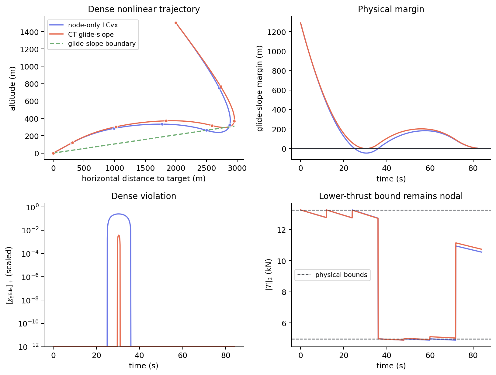
The thrust panel marks the scope of the experiment. The CT trajectory retains a $77.844\,\mathrm N$ inter-sample shortfall in the physical lower-thrust bound because that family remains nodal. The experiment therefore treats glide slope continuously; it does not establish continuous-time feasibility for every rocket constraint.
Cart-pole: dynamic consistency and inter-sample feasibility
Cart-pole enters directly at the SCvx stage: it has smooth nonlinear dynamics, but this experiment has no LCvx-style tight control relaxation. With $x=[p,\theta,\dot p,\dot\theta]^\top$, force $F$, cart mass $M$, pole mass $m$, and pole length $\ell$, the direct input coefficient in angular acceleration is
\[\frac{\partial\ddot\theta}{\partial F} =-\frac{\cos\theta} {\ell\left(M+m\sin^2\theta\right)}.\]During the swing-up, the dynamics can amplify accumulated integration and transcription errors. This is especially true when the pole moves from angle $\pi/2$ toward $\pi$, and particularly near $\pi/2$, where the cart has poor instantaneous authority over the pole. The light-blue curve in the trajectory figure below shows the one-model open-loop rollout missing the swing-up after this sensitive region. Russ Tedrake’s trajectory-optimization notes and code give a detailed explanation of why trajectory stabilization matters. In this region, even a small mismatch between the simulated state and the nominal trajectory can be amplified significantly, causing the open-loop rollout to miss the swing-up.
This coefficient describes instantaneous input authority, not loss of controllability at $\pi/2$. A dynamically consistent open-loop trajectory also serves a different purpose from feedback stabilization. Integration error, shooting defect, inter-sample constraint violation, and open-loop sensitivity are therefore evaluated as separate properties.
The experiment uses an unwrapped target $\theta(t_f)=\pi$, $t_f=5\,\mathrm{s}$, 16 knots, ZOH force, and the track limit $\lvert p(t)\rvert\le0.28\,\mathrm m$. A deliberately coarse 15-interval nonlinear solve identifies a swing-up family. After resampling and nonlinear rollout, this initializer has a scaled terminal error of $4.682\times10^{-2}$ and reaches $\lvert p\rvert=0.313\,\mathrm m$. Only its primal state and control supply the common reference; no multiplier or barrier state is transferred.
| Metric | One affine model | Node-only SCvx | CT-SCvx |
|---|---|---|---|
| Scaled terminal error | $7.118\times10^{-1}$ | $1.205\times10^{-5}$ | $1.181\times10^{-5}$ |
| Nodal track violation | — | $0$ to reported precision | $0$ to reported precision |
| Dense track violation | $38.6\,\mathrm{mm}$ | $38.7\,\mathrm{mm}$ | $1.864\,\mathrm{mm}$ |
One affine model does not predict the nonlinear open-loop swing-up: the rollout misses the terminal angle by $-1.047\,\mathrm{rad}$, approximately $-\pi/3$. Repeated SCvx reduces the scaled dynamic defect to $4.296\times10^{-10}$ and the virtual-control norm to $1.178\times10^{-13}$; it takes 8 accepted outer steps and 24 convex solves.
The corresponding CT-SCvx values are a $4.155\times10^{-10}$ physical-state defect, a $7.116\times10^{-9}$ augmented-state defect, 53 accepted steps, and 96 convex solves. Its maximum $y$ increment is $9.668\times10^{-7}$ and its normalized accumulated violation is $9.667\times10^{-7}$.
SCvx has repaired local model agreement and dynamic consistency, but its track condition remains nodal. The node-only trajectory satisfies all 16 sampled bounds while leaving the track by $38.7\,\mathrm{mm}$ between them. With the same dynamics, horizon, grid, control hold, initial reference, scaling, objective, and cone solver, CT-SCvx reduces the dense diagnostic to $1.864\,\mathrm{mm}$. Its accumulated violation remains positive, consistent with the relaxed constraint and finite numerical tolerances.
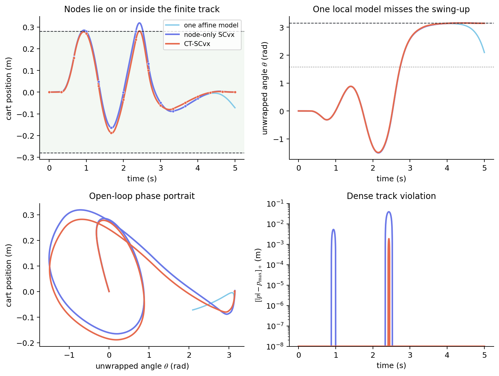
The solve counts provide algorithmic context rather than a speed comparison. The outer methods use different globalization rules, and this implementation is not a matched performance benchmark. A runtime claim would require controlled implementations, repeated measurements, and comparable stopping conditions.
Comparison of LCvx, SCvx, and CT-SCvx
| Method | Convexified object | Solves | Defensible result |
|---|---|---|---|
| LCvx | A structured control set through a tight lift | One, or a small fixed sequence | Global optimum of the stated structured model, under the losslessness assumptions |
| SCvx | A safeguarded local model of nonlinear residuals | Repeated | Stationary accumulation points of the penalized finite problem, under compactness and regularity assumptions |
| CT-SCvx | An augmented flow and its convex-composite local model | Repeated | Penalized-problem stationarity, conditional KKT recovery, and a continuous-time path interpretation under the reformulation assumptions |
The limits follow the same progression. LCvx applies to a narrow geometry and does not remove transcription error. SCvx has a local solution concept and may enforce path constraints only at nodes. CT-SCvx still uses finite control parameterizations, numerical flow integration, positive tolerances, and local stationarity for nonconvex problems.
The common research style is to expose the convex structure that remains, then make a precise claim about what that structure preserves. At first, convexification acts on the feasible set; then on the local model; finally on the finite representation of a continuous-time claim.
References
-
B. Açıkmeşe and L. Blackmore, “Lossless Convexification of a Class of Optimal Control Problems with Non-Convex Control Constraints”, Automatica, 2011. See Sec. 2, Eqs. (1), (3)–(10), Theorem 2, and the PMP argument in Eqs. (11)–(22).
-
B. Açıkmeşe, J. M. Carson III, and L. Blackmore, “Lossless Convexification of Nonconvex Control Bound and Pointing Constraints of the Soft Landing Optimal Control Problem”, IEEE Transactions on Control Systems Technology, 2013. See Secs. II–IV, Problems 1–4, Theorem 1, and Eqs. (33)–(36).
-
Y. Mao, M. Szmuk, and B. Açıkmeşe, “Successive Convexification of Non-Convex Optimal Control Problems and Its Convergence Properties”, arXiv v3, 2016. See Sec. II, Eqs. (1)–(9), Algorithm 1, and Sec. III.
-
M. Szmuk and B. Açıkmeşe, “Successive Convexification for 6-DoF Mars Rocket Powered Landing with Free-Final-Time”, 2018. See Secs. II–III, Problems 1–2, Eqs. (14)–(27), and Algorithm 1.
-
Y. Mao, M. Szmuk, X. Xu, and B. Açıkmeşe, “Successive Convexification: A Superlinearly Convergent Algorithm for Non-convex Optimal Control Problems”, arXiv v2, 2018/2019. See Secs. 2–4, especially Theorems 3.9, 3.13, and 4.7, together with Ref. 6.
-
Y. Luo, P. Elango, and B. Açıkmeşe, “Remarks on ‘Successive Convexification: A Superlinearly Convergent Algorithm for Non-convex Optimal Control Problems’”, arXiv v2, 2024. See Sec. 2 for the corrections and Sec. 3 for the stronger whole-sequence result.
-
P. Elango et al., “Successive Convexification for Trajectory Optimization with Continuous-Time Constraint Satisfaction”, 2024. See Lemma 2, Corollary 3, Lemma 10, Theorem 14, Algorithm 1, and the stationarity/KKT results in Secs. 4–5.
Reference implementations
-
The pinned CT-SCvx implementation directly accompanies Ref. 7.
-
SCPToolbox.jl is a later general-purpose reference implementation; its current branch is not the historical code for Refs. 3–4.
-
The executable notebook accompanies this article.