ADMM and Proportional–Integral Projected Gradient Methods

The ADMM code for this post is in splitQP; the PIPG notebook is in splitQP/pipg.

ADMM and the proportional–integral projected-gradient family are first-order primal–dual methods for constrained optimization. Both combine a primal update with a constraint-space state driven by residuals, and both rely on simple projections whenever the problem representation permits them. Their principal computational difference lies in the primal update: ADMM evaluates a proximal subproblem—an equality-constrained quadratic program in OSQP—whereas PIPGeq takes an explicit projected-gradient step and returns the constraint correction through $G^\top$. A reusable factorization can make the former inexpensive over a fixed problem family; the latter removes the linear solve from its online iteration, but exposes the iteration more directly to scaling and geometry.

The discussion below begins with the augmented Lagrangian, specializes ADMM to quadratic programs, and then develops the paper lineage $\text{PIPGeq}\rightarrow\text{PIPG}\rightarrow\text{xPIPG}$. This ordering is not a claim that PIPG historically descends from ADMM. It places two related primal–dual constructions on the same problem so that their states, operators, and computational costs can be compared without changing the model.

Dual ascent and the augmented Lagrangian

Consider an equality-constrained convex problem

\[\min_x f(x) \qquad\text{subject to}\qquad Ax=b.\]

Its Lagrangian and dual function are

\[\mathcal L(x,y)=f(x)+y^\top(Ax-b), \qquad d(y)=\inf_x\mathcal L(x,y).\]

When a minimizer $x^+(y)$ exists and $d$ is differentiable, $\nabla d(y)=Ax^+(y)-b$. Dual ascent therefore alternates between an exact primal minimization and a residual update:

\[\begin{aligned} x^{k+1}&\in\arg\min_x\mathcal L(x,y^k),\\ y^{k+1}&=y^k+\alpha_k(Ax^{k+1}-b). \end{aligned}\]

The multiplier already has a concrete dynamical interpretation. For a constant step, it is the initial multiplier plus a running sum of equality residuals. This accumulation is useful, but the unaugmented primal minimization may be nonunique, poorly conditioned, or even unbounded for intermediate multipliers.

The augmented Lagrangian adds a quadratic penalty:

\[\mathcal L_\rho(x,y) =f(x)+y^\top(Ax-b)+\frac{\rho}{2}\lVert Ax-b\rVert_2^2.\]

The method of multipliers uses

\[\begin{aligned} x^{k+1}&\in\arg\min_x\mathcal L_\rho(x,y^k),\\ y^{k+1}&=y^k+\rho(Ax^{k+1}-b). \end{aligned}\]

The penalty regularizes the primal step and makes constraint violation visible inside it. The same term also couples all variables that appear in $Ax-b$. This is the point at which alternating minimization becomes useful.

ADMM

ADMM applies the augmented-Lagrangian idea to a separable problem

\[\begin{aligned} \min_{x,z}\quad &f(x)+g(z),\\ \text{subject to}\quad&Ax+Bz=c. \end{aligned}\]

With residual $r=Ax+Bz-c$ and scaled multiplier $u=y/\rho$, completing the square gives

\[y^\top r+\frac{\rho}{2}\lVert r\rVert^2 =\frac{\rho}{2}\lVert r+u\rVert^2 -\frac{\rho}{2}\lVert u\rVert^2.\]

One scaled ADMM iteration is then

\[\begin{aligned} x^{k+1} &\in\arg\min_x f(x)+\frac{\rho}{2} \lVert Ax+Bz^k-c+u^k\rVert^2,\\ z^{k+1} &\in\arg\min_z g(z)+\frac{\rho}{2} \lVert Ax^{k+1}+Bz-c+u^k\rVert^2,\\ u^{k+1} &=u^k+Ax^{k+1}+Bz^{k+1}-c. \end{aligned}\]

The first two lines are proximal subproblems evaluated in sequence. The last line integrates the splitting residual:

\[u^k=u^0+\sum_{i=1}^k r^i.\]

This is the first structural resemblance to PIPG: both methods carry a constraint-space state with memory. The residuals are nevertheless different. ADMM accumulates the agreement error between split variables, whereas PIPGeq will accumulate the original equality residual $Gz-g$ directly. Their primal maps are also different, so the states should not be identified merely because both are residual sums.

For generic ADMM, the cost of an iteration is the cost of the two proximal operators. They may be scalar formulas, projections, linear solves, or complete inner optimization problems. Statements about ADMM’s linear algebra are therefore meaningful only after a particular splitting has been chosen.

The conventional primal residual is

\[r_{\mathrm{prim}}^{k+1} =Ax^{k+1}+Bz^{k+1}-c,\]

while the change in the second block produces the familiar dual residual

\[r_{\mathrm{dual}}^{k+1} =\rho A^\top B(z^{k+1}-z^k).\]

These are finite-iteration expressions of primal feasibility and stationarity, not merely measures of whether the iterates have stopped moving.

ADMM specialized to a quadratic program

OSQP considers the convex quadratic program

\[\begin{aligned} \min_x\quad&\frac12x^\top Px+q^\top x,\\ \text{subject to}\quad&l\le Ax\le u, \end{aligned}\]

where $P\succeq0$. Introducing $z=Ax$ separates the quadratic objective from the interval $[l,u]$. Projection of $z$ is then a componentwise clip; the other ADMM subproblem is an equality-constrained QP. Writing the possibly diagonal OSQP penalty as $R$, its optimality conditions reduce to

\[\begin{bmatrix} P+\sigma I&A^\top\\ A&-R^{-1} \end{bmatrix} \begin{bmatrix} \widetilde x^{k+1}\\ \nu^{k+1} \end{bmatrix} = \begin{bmatrix} \sigma x^k-q\\ z^k-R^{-1}y^k \end{bmatrix},\]

where $R$ is a positive diagonal penalty matrix. The quasi-definite coefficient matrix is independent of the iterates. A direct implementation factors it once and reuses the factors for forward and backward substitution. If $P$, $A$, $\sigma$, or $R$ changes numerically, the numerical factorization changes as well, although an unchanged sparsity pattern can preserve symbolic analysis.

Eliminating $\nu$ gives the positive-definite alternative

\[(P+\sigma I+A^\top R A)\widetilde x^{k+1} =\text{iteration-dependent right-hand side}.\]

This system can also be solved iteratively. That avoids a direct factorization, but it does not remove the linear-system solve; it moves the solve into an inner iteration.

In a dense fixed-matrix implementation, this factor can be reused while $q,l,u$ vary. Each online iteration then applies $A^\top$ and $A$, performs an interval projection, and uses one forward and one backward triangular solve. This is a favorable regime for direct ADMM by construction: the coupled inverse map is paid for once and applied repeatedly through its factors.

For this QP form, it is natural to monitor the KKT residuals directly:

\[r_{\mathrm{prim}}=Ax-z, \qquad r_{\mathrm{dual}}=Px+q+A^\top y.\]

The penalty $R$ is simultaneously an ADMM metric and a form of constraint scaling. A single scalar $\rho$ sets one compromise for every row; a diagonal $R$ can compensate for rows with different units or magnitudes. Adaptive residual balancing changes this metric during the solve, but a direct method must then pay for a new numerical factorization. Preconditioning is already part of the algorithm’s effective geometry, well before PIPG enters the discussion.

PIPGeq

The foundational PIPGeq paper begins from a closely related problem:

\[\begin{aligned} \min_{z\in Z}\quad&\frac12z^\top Pz+q^\top z,\\ \text{subject to}\quad&Gz=g, \end{aligned}\]

with $P\succeq0$, $G\in\mathbb R^{m\times n}$, and a closed convex set $Z$ whose Euclidean projection is inexpensive. In model predictive control, $Gz=g$ typically represents dynamics, while $Z$ is a Cartesian product of state and input sets.

There is one notation change worth making explicit. The 2020 PIPGeq paper calls the objective Hessian $H$ and the equality operator $G$; the later conic papers call the objective Hessian $P$ and the affine operator $H$. I use $P$ for objective curvature throughout, retain $G$ for the equality-only problem, and switch to $H$ only when the general cone is introduced.

Applied to this problem, an ADMM splitting uses two copies of the primal variable: one is constrained by $Gz=g$, and the other by $z\in Z$. The first subproblem in the PIPGeq paper has the KKT system

\[\begin{bmatrix} P+\tau^{-1}I&G^\top\\ G&0 \end{bmatrix} \begin{bmatrix}y^{k+1}\\\nu^{k+1}\end{bmatrix} = \begin{bmatrix} -q-\tau^{-1}(w^k-z^k)\\g \end{bmatrix}.\]

Here $y$ is the equality-constrained primal copy and $\nu$ is its multiplier. When $P$ and $G$ are fixed, this system is a good candidate for an offline factorization. When they change from one online problem to the next, the same step requires new linear algebra. PIPGeq changes this particular primal update:

\[\begin{aligned} v^k &=w^k+\beta(Gz^k-g),\\ z^{k+1} &=\Pi_Z\!\left[ z^k-\alpha(Pz^k+q+G^\top v^k) \right],\\ w^{k+1} &=w^k+\beta(Gz^{k+1}-g). \end{aligned}\]

The name is literal. With a constant $\beta$,

\[w^k=w^0+\beta\sum_{i=1}^k(Gz^i-g),\]

so $w^k$ is the discrete integral of the equality residual. The term $\beta(Gz^k-g)$ is the instantaneous proportional correction, and $v^k$ is their sum. Finally, $G^\top v^k$ maps this constraint-space signal back to the primal space, where it corrects the objective gradient.

This interpretation is more precise than saying that PIPGeq merely “uses feedback.” Its primal step contains three visible directions:

\[-\alpha(Pz+q), \qquad -\alpha G^\top\beta(Gz-g), \qquad -\alpha G^\top w.\]

They are respectively the projected-gradient, proportional, and integral contributions before projection onto $Z$.

The same decomposition can be read directly through the augmented Lagrangian:

\[\begin{aligned} Pz^k+q+G^\top v^k =\nabla_z\biggl( &\frac12z^\top Pz+q^\top z +\langle w^k,Gz-g\rangle\\ &+\frac{\beta}{2}\lVert Gz-g\rVert^2 \biggr)\bigg|_{z=z^k}. \end{aligned}\]

The proportional term is therefore not an additional heuristic correction; it is the gradient of the quadratic penalty on the current equality residual. The integral state supplies the multiplier term. This does not turn PIPGeq into ADMM: ADMM minimizes augmented proximal subproblems for a chosen splitting, whereas PIPGeq evaluates this gradient once and projects. It does identify the computational fork precisely. One method applies a coupled inverse map; the other replaces that map by a scalar-step forward approximation.

For the constant-step theorem in the original paper, if $P\preceq\lambda I$ and $G^\top G\preceq\sigma I$, the steps satisfy

\[\alpha(\lambda+\sigma\beta)=1.\]

The experiment below uses

\[\begin{aligned} \min_{z\in[-1,1]^2}\quad& \frac12z^\top \begin{bmatrix}4&0\\0&1\end{bmatrix}z +\begin{bmatrix}-3&-1\end{bmatrix}z,\\ \text{subject to}\quad&[1,1]z=0.5. \end{aligned}\]

The solution is $z^\star=(0.5,0)$ with $f^\star=-1$. Projected gradient sees the box but not the affine line and therefore converges to the optimum of the wrong problem. ADMM and PIPGeq approach the same constrained solution using different primal maps. The second panel evaluates all three PIPGeq directions at one common iterate; their sum is the trial step before box projection.

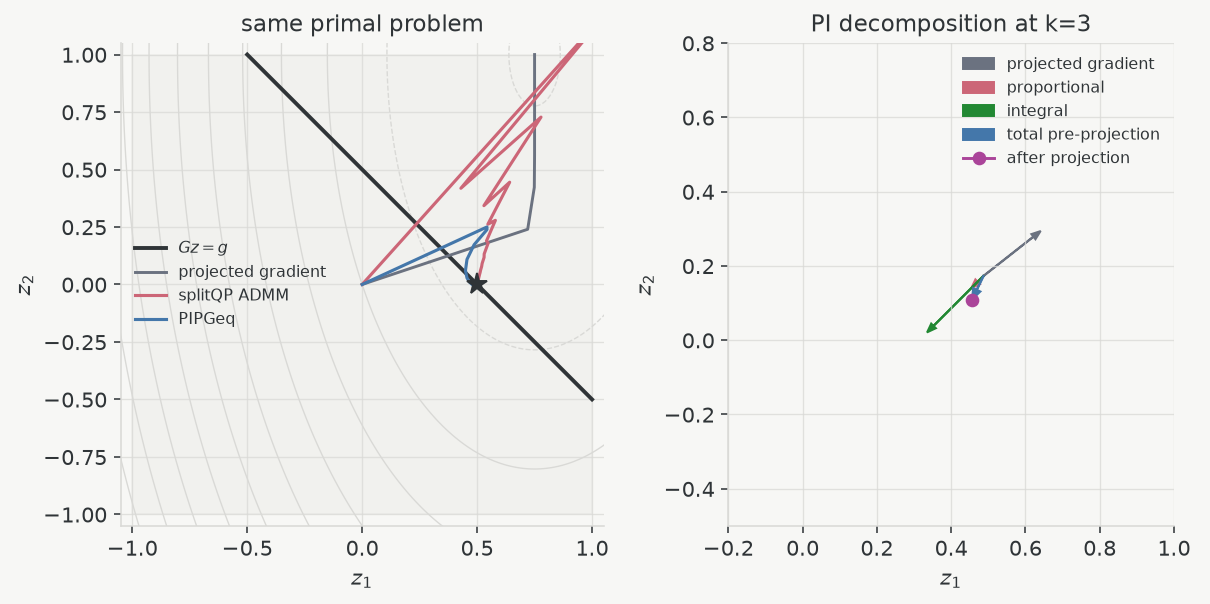
On this example, $\lambda=4$, $\sigma=\lVert G\rVert^2=2$, $\beta=\sqrt2$, and $\alpha\approx0.146447$. PIPGeq reaches an equality residual below $10^{-6}$ in about 25 iterations; the factor-reusing ADMM baseline terminates after 104 iterations at its stricter $10^{-9}$ absolute and relative tolerances. These counts describe the chosen parameters and stopping rules, not an intrinsic ordering of the methods.

The online PIPGeq formula contains products with $P$, $G$, and $G^\top$, plus one projection onto $Z$. It contains no linear-system solve. This qualification matters: norm estimation, preconditioning, and code generation are setup work, and $\Pi_{Z}$ may itself be an optimization problem unless $Z$ has a simple product structure. PIPGeq is inexpensive only when these operators are inexpensive.

General conic PIPG

PIPGeq treats $Gz-g=0$. General PIPG considers

\[\begin{aligned} \min_{z\in D}\quad&f(z),\\ \text{subject to}\quad&Hz-g\in K, \end{aligned}\]

where $D\subseteq\mathbb R^n$ is closed and convex and $K\subseteq\mathbb R^m$ is a closed convex cone. The paper uses the polar cone

\[K^\circ =\{w:\langle w,y\rangle\le0\ \text{for every }y\in K\}.\]

This sign convention is not cosmetic. If $K^{\ast}={w:\langle w,y\rangle\ge0}$ denotes the usual dual cone, then $K^\circ=-K^{\ast}$. Thus

\[(\mathbb R_+^m)^\circ=\mathbb R_-^m, \qquad K_{\mathrm{soc}}^\circ=-K_{\mathrm{soc}}, \qquad \{0\}^\circ=\mathbb R^m.\]

The saddle representation is

\[\min_{z\in D}\ \max_{w\in K^\circ} f(z)+\langle Hz-g,w\rangle.\]

Consequently, the constraint correction must remain in $K^\circ$. PIPG does this with

\[\begin{aligned} w^{j+1} &=\Pi_{K^\circ}\!\left[v^j+\beta^j(Hz^j-g)\right],\\ z^{j+1} &=\Pi_D\!\left[ z^j-\alpha^j\bigl(\nabla f(z^j)+H^\top w^{j+1}\bigr) \right],\\ v^{j+1} &=w^{j+1}+\beta^jH(z^{j+1}-z^j). \end{aligned}\]

The first line adds the current conic residual and projects the correction onto the admissible multiplier cone. The second returns that correction through $H^\top$. The final line predicts the correction associated with the new primal point. The pair of dual-side updates is therefore a projected prediction–correction form of the PI state.

For $K=\mathbb R_{+}^{m}$, a negative component of $Hz-g$ is a violation and drives the corresponding correction into the negative orthant; positive feasible slack moves it back toward zero. The polar projection prevents a multiplier with the wrong sign. For an SOC, the same selection is geometric rather than componentwise.

If $K={0}$, the polar projection is the identity. Combining the first and third lines gives

\[v^{j+1}=v^j+\beta^j(Hz^{j+1}-g),\]

which recovers the equality integral update. For product cones, all projections separate blockwise. Moreau’s decomposition is particularly convenient:

\[\Pi_{K^\circ}(a)=a-\Pi_K(a).\]

Orthants and second-order cones therefore retain closed-form projections. An arbitrary intersection or rotated polytope need not.

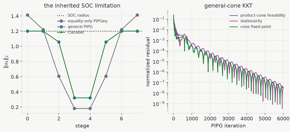
The trajectory experiment below adds a genuine second-order-cone bound on the control norm while keeping the affine dynamics and box bounds unchanged. Equality-only PIPGeq satisfies the dynamics but violates the SOC radius at the outer stages. General PIPG agrees with the independent conic reference and drives feasibility, stationarity, and the cone fixed-point residual down together.

Constant-step PIPG and PDHG

General PIPG is closely related to a constant-step forward variant of PDHG. For constant $\beta$, the final PIPG line from the preceding iteration gives

\[v^j=w^j+\beta H(z^j-z^{j-1}).\]

Substitution into the next polar projection yields

\[\begin{aligned} w^{j+1} &=\Pi_{K^\circ}\!\left[ w^j+\beta H(z^j-z^{j-1})+\beta(Hz^j-g) \right]\\ &=\Pi_{K^\circ}\!\left[ w^j+\beta\{H(2z^j-z^{j-1})-g\} \right]. \end{aligned}\]

Together with the projected primal-forward step, and after an index shift, this is the constant-step PDHG form displayed in the PIPG paper. The statement is exact but narrow: it does not identify every method called PDHG with PIPG, and it does not make varying-step PIPG or relaxed xPIPG the same iteration.

ADMM is likewise related to Douglas–Rachford splitting, but through a different monotone inclusion and different resolvents. These methods share primal–dual state, projections, residuals, and fixed-point language; they should still be distinguished by the operator evaluated at each iteration.

xPIPG

For the quadratic cone problem

\[\begin{aligned} \min_{z\in D}\quad&\frac12z^\top Pz+q^\top z,\\ \text{subject to}\quad&Hz-g\in K, \end{aligned}\]

xPIPG writes the iteration in terms of relaxed primal and dual states $(\xi^j,\eta^j)$:

\[\begin{aligned} z^{j+1} &=\Pi_D\!\left[ \xi^j-\alpha(P\xi^j+q+H^\top\eta^j) \right],\\ w^{j+1} &=\Pi_{K^\circ}\!\left[ \eta^j+\beta\{H(2z^{j+1}-\xi^j)-g\} \right],\\ \xi^{j+1} &=(1-\rho)\xi^j+\rho z^{j+1},\\ \eta^{j+1} &=(1-\rho)\eta^j+\rho w^{j+1}. \end{aligned}\]

Here $z^{j+1}$ and $w^{j+1}$ are projected base points; $\xi^{j+1}$ and $\eta^{j+1}$ are the fixed-point states carried to the next iteration. With $\rho=1$, the base points become the next states and the unrelaxed PIPG/PDHG representation is recovered. Values $1<\rho<2$ extrapolate the fixed-point map. The argument $2z^{j+1}-\xi^j$ is the reflection of the incoming primal state through its projected point, so the dual projection sees the newest primal correction. This reflected coupling and the relaxation by $\rho$ are fixed-point operations, not Nesterov momentum.

The basic sufficient condition is

\[\alpha\bigl(\lVert P\rVert+\beta\lVert H\rVert^2\bigr)<1, \qquad 0<\rho<2.\]

Writing $\beta=\omega\alpha$ gives the equivalent upper bound

\[0<\alpha< \frac{2} {\sqrt{\lVert P\rVert^2+4\omega\lVert H\rVert^2} +\lVert P\rVert}.\]

The open inequalities are important. An implementation normally estimates $\lVert H\rVert$ and keeps a numerical safety margin; the power iteration used for this estimate belongs to setup, not to the recurring xPIPG kernel.

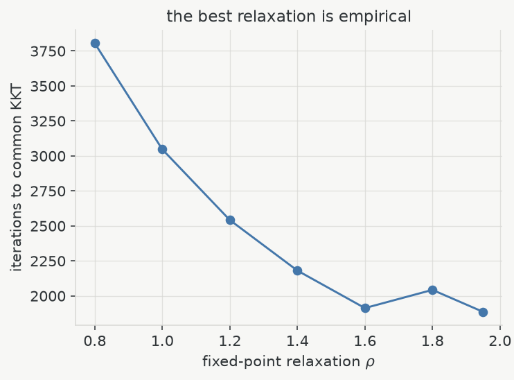
Relaxation changes the transient without changing the underlying fixed points. There is no universal best $\rho$. On the trajectory problem, the same $\alpha$ and $\beta$ were used for $\rho\in{0.8,1.0,1.2,1.4,1.6,1.8,1.95}$. The measured iteration counts to a common KKT target were respectively $3804,3046,2541,2180,1912,2042,$ and $1885$. The best value on this finite grid was $1.95$; the nonmonotone change between $1.6$ and $1.8$ is enough to rule out treating a value reported by one implementation as a universal constant.

Iterate differences and infeasibility

If the conic problem has a primal–dual solution, the xPIPG fixed-point state can converge and consecutive base-point differences approach zero. When no fixed point exists, averaged-operator theory allows the differences to approach a nonzero minimal-displacement direction instead. For diagnostics, it is convenient to remove the primal, dual, and relaxation scales:

\[\widehat z^k=\frac{z^{k+1}-z^k}{\alpha\rho}, \qquad \widehat w^k=\frac{w^{k+1}-w^k}{\beta\rho}, \qquad d_z^k=\lVert\widehat z^k\rVert, \quad d_w^k=\lVert\widehat w^k\rVert.\]

Positive rescaling does not change cone membership or the sign of a separation test. The magnitudes $d_{z}^k$ and $d_{w}^k$ are nevertheless only a first indication. A limiting dual direction $\bar w$ certifies primal infeasibility only if it belongs to $K^\circ$ and strictly separates the attainable residuals from $K$:

\[\bar w\in K^\circ, \qquad \inf_{z\in D}\langle Hz-g,\bar w\rangle>0.\]

For a box $D$, the infimum is evaluated exactly by choosing a lower or upper bound according to the sign of each component of $H^\top\bar w$. For a general set, validating the certificate requires a support-function or linear- minimization oracle, which may itself be nontrivial.

A candidate primal direction $\bar z$ certifies dual infeasibility or unboundedness only after the corresponding recession and improvement tests:

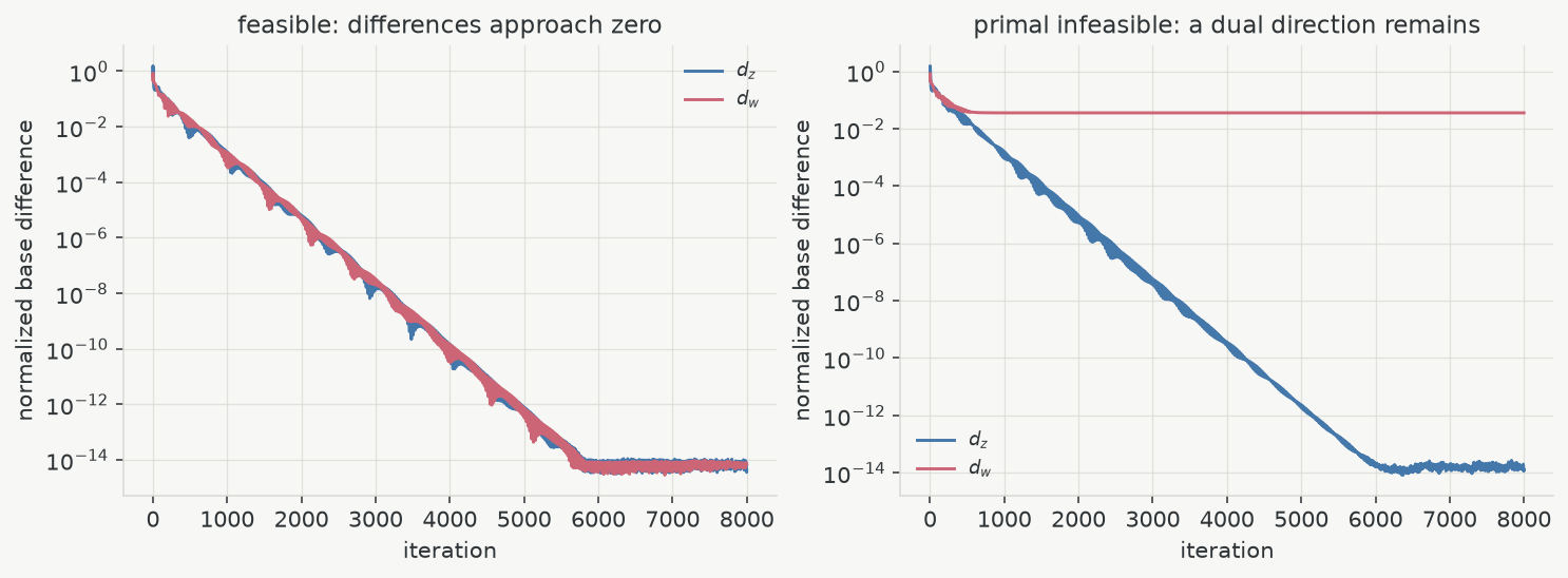
\[\bar z\in\operatorname{rec}D, \qquad P\bar z=0, \qquad H\bar z\in K, \qquad q^\top\bar z<0.\]

The matched experiment keeps the same dimensions, cone blocks, objective, and steps. Only the conic radius changes. In the feasible instance both normalized differences fall to about $10^{-14}$ and the final KKT residual is $7.9\times10^{-16}$. In the primal-infeasible instance the primal difference vanishes while the dual difference remains near $3.56\times10^{-2}$. The normalized direction has polar-cone distance below $10^{-15}$ and separation margin $3.56\times10^{-2}$.

A separate one-dimensional problem with $P=0$, $q=-1$, no affine constraint, and $D=\mathbb R$ yields the direction $\bar z=1$, for which $P\bar z=0$ and $q^\top\bar z=-1$. This distinguishes the dual-infeasible or unbounded case from primal infeasibility. At finite iteration counts, a solver should consequently distinguish converged feasible, likely primal infeasible, likely dual infeasible or unbounded, maximum iterations, stagnation, and numerical ambiguity.

OSQP also extracts infeasibility information from successive differences. The shared minimal-displacement language does not make OSQP’s ADMM map identical to xPIPG; each method still validates certificates in its own canonical variables and scaling.

Preconditioning

For an explicit primal–dual method, the stability condition already reveals the geometric bottleneck:

\[\alpha\bigl(\lVert P\rVert+\beta\lVert H\rVert^2\bigr)<1.\]

A large eigenvalue of $P$ or singular value of $H$ restricts the one global primal step. A poorly scaled constraint operator also makes one dual step too large for some directions and too small for others. Stability alone is not enough: after a conservative step is chosen, small singular directions may still progress slowly.

ADMM sees the same coordinates through a different operator. Its penalty and scaling determine the conditioning of $P+\sigma I+A^\top R A$ or of the quasi-definite KKT matrix. PIPG sees them through forward products and a global step bound. In both cases preconditioning changes the metric in which the iteration measures progress; it is not merely a final round of scalar tuning.

Diagonal scaling and Ruiz equilibration

Scalar objective scaling changes the relative magnitude of objective and constraint feedback without changing the minimizer. A scalar primal–dual step ratio can improve this balance, but neither operation removes anisotropy among rows and columns.

Diagonal equilibration is more expressive while remaining compatible with sparse products. Modified Ruiz equilibration repeatedly balances rows and columns of a KKT representation. In an ADMM implementation it improves the linear system and the residual scales; in PIPG it changes the spectral geometry that limits $\alpha$ and $\beta$. The transform must still be propagated to warm starts, residuals, multipliers, and termination tolerances.

QR preconditioning for equalities

For a strongly convex equality-constrained problem with full-row-rank $H$, let

\[H^\top=QR\]

be a thin QR factorization. The QR preconditioner replaces $Hz=g$ by

\[\widehat H z=\widehat g, \qquad \widehat H=\eta Q^\top, \qquad \widehat g=\eta R^{-\top}g.\]

The feasible set is unchanged, while every singular value of $\widehat H$ is $\eta$. The scaling proposed in the paper is

\[\eta= \sqrt{\lambda_{\max}(P)\lambda_{\min}(P) +\lambda_{\min}^2(P)}.\]

Geometrically, nearly parallel equality normals require the integral state to build very different coefficients before $H^\top w$ can move in all primal directions. QR replaces those normals by orthogonal, equally scaled ones. In the two-dimensional example below, the raw singular values are approximately $1.414$ and $0.00707$; after QR both are $2.236$. The equality-KKT condition number falls from $8.9\times10^4$ to $5$, and xPIPG reaches the target in 37 iterations where the raw representation does not reach it within 12,000.

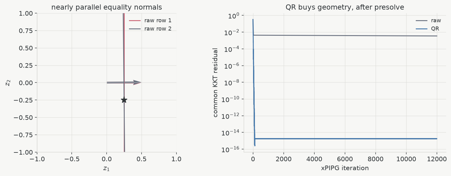
This result is deliberately narrow. QR requires full-row-rank equalities, computes a factorization and triangular solve during presolve, and often fills in a sparse constraint matrix. It is not a structure-preserving generic conic preconditioner.

Hypersphere preconditioning and projection structure

If $P=R^\top R\succ0$, define new coordinates

\[\xi=Rz, \qquad z=R^{-1}\xi.\]

The quadratic Hessian becomes the identity and the constraint operator becomes $HR^{-1}$. Cone-compatible block-row normalization can then scale equality and orthant rows individually, but every row within an SOC block must receive the same scalar so that the cone itself is preserved.

The primal set becomes

\[\widehat D=RD.\]

This is the decisive qualification. If $D$ is a box and $R$ is a general dense matrix, $RD$ is a rotated parallelotope. Componentwise clipping is no longer its Euclidean projection. Whitening has improved the Hessian while destroying the inexpensive primal operator that made PIPG attractive. Diagonal or suitable block-diagonal Hessians can avoid this conflict; an arbitrary Cholesky factor cannot.

After compatible whitening and row normalization, the newer preconditioning paper also chooses an objective scalar. If $\sigma_{\min}=\lambda_{\min}(\widehat H\widehat H^\top)$, the derived scale is

\[\lambda^\star=\sqrt{\frac{\sigma_{\min}}{2}},\]

and the corresponding PIPG ratio is written as

\[\omega^\star =\lambda\sqrt{\frac{2}{\sigma_{\min}}}, \qquad \frac{\beta}{\alpha}=\omega^2.\]

Objective scaling and the primal–dual step ratio therefore describe the same relative degree of freedom in this construction; they should not be tuned as if they were independent.

The following experiment writes one trajectory QP in eight mathematically equivalent representations. Scalar ratio tuning reduces 1395 iterations to 853 without changing the KKT condition number. Modified Ruiz needs 184; whitening alone needs 357; QR needs 886 and raises operator density from $0.067$ to $0.288$. The complete projection-compatible hypersphere, block-row, and objective-scale construction needs 130 iterations. These numbers are not a ranking of preconditioners in general—the QR example above already shows a regime in which QR is much stronger—but they expose why no single condition number or scalar parameter describes the whole iteration.

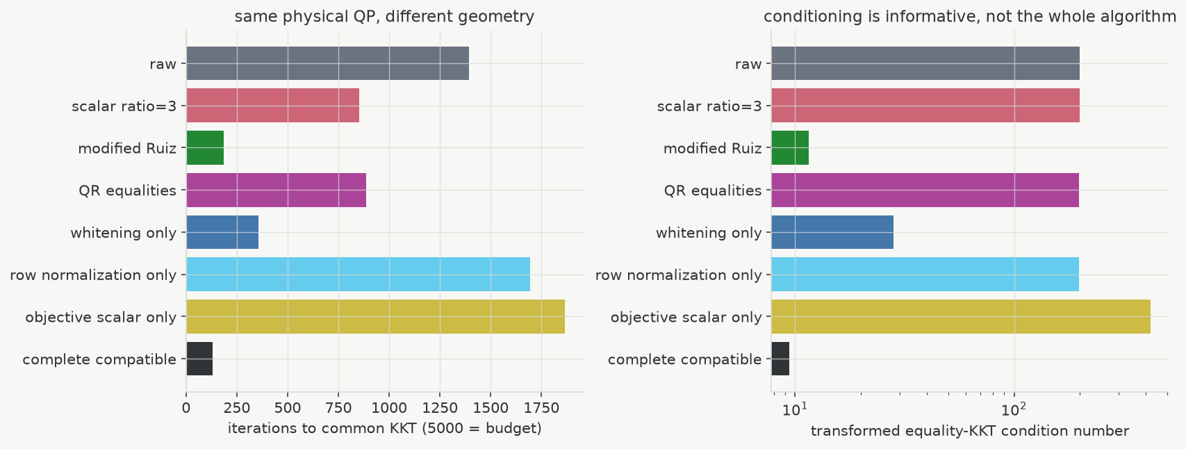
The practical principle is simple: a preconditioner is useful only when it improves geometry without making the required projections or operator applications more expensive than the original problem.

Per-iteration operations

The recurring work is easier to compare after separating it from setup:

Method	Persistent state	Recurring online work	Setup that may be reused
Direct QP ADMM	primal, split, and dual states; cached factor	$A$, $A^\top$, one interval projection, forward/backward triangular solves	KKT or positive-definite factorization
PIPGeq	$z$, integral state $w$, optionally cached $Gz-g$	one product each with $P$, $G$, and $G^\top$; one projection onto $Z$	norm estimates and any scaling
PIPG	$z$, prediction state $v$, projected correction $w$	one product each with $P$, $H$, and $H^\top$ when $Hz$ is cached; projections onto $D$ and $K^\circ$	norm estimates and conic scaling
xPIPG	relaxed states $\xi,\eta$ and base points $z,w$	one $P$, one $H$, one $H^\top$, two projections, and relaxation	norm estimates, step selection, preconditioning

The phrase “no linear-system solve” applies to the explicit online PIPG/xPIPG kernel under this representation. It does not include QR or Cholesky preconditioning, singular-value estimation, compilation, or a projection that internally solves another optimization problem. Conversely, a direct ADMM iteration reuses rather than repeats its factorization, and its triangular solves may be exceptionally efficient for a small fixed system.

Warm starts are natural for all of these fixed-point states. For ADMM one warms the primal, split, and dual variables. For xPIPG one must distinguish the relaxed states $(\xi,\eta)$ from the projected base points $(z,w)$ and transform the dual state consistently if the constraints have been scaled.

Setup cost and amortization

A timing comparison is meaningful only if both methods use the same physical residuals and neither is charged selectively for setup. Data construction, factorization or norm estimation, compilation, and online execution are therefore separated, and both methods stop on the same original-coordinate KKT criterion. An independent reference solution is used to check the result, not to decide when either iteration stops.

Two regimes were measured. In the changing-matrix regime, varying the dynamics time step changes $P$ or $A$ while preserving array shapes. ADMM repeats a $1.37$–$2.55$ ms setup and a $1.90$–$6.87$ ms online solve; xPIPG repeats a $0.65$–$0.72$ ms norm/step setup and a $2.57$–$3.15$ ms online solve. Both terminate at an original-coordinate KKT residual of approximately $10^{-5}$. The ranges overlap, so even this small example does not support a categorical claim.

With fixed matrices, both methods reuse setup and consecutive targets warm-start from the preceding terminal state. At family size $B=1$, post-compilation online time is about $3.1$ ms for either method; including setup gives $4.3$ ms for ADMM and $3.8$ ms for xPIPG. At $B=128$, the corresponding totals are $143.4$ ms and $115.2$ ms in this CPU experiment, although xPIPG performs 63,780 iterations against ADMM’s 33,061. Here the cheaper explicit kernel offsets a higher iteration count. A different factorization backend, sparsity pattern, accuracy target, or processor can move the crossing point.

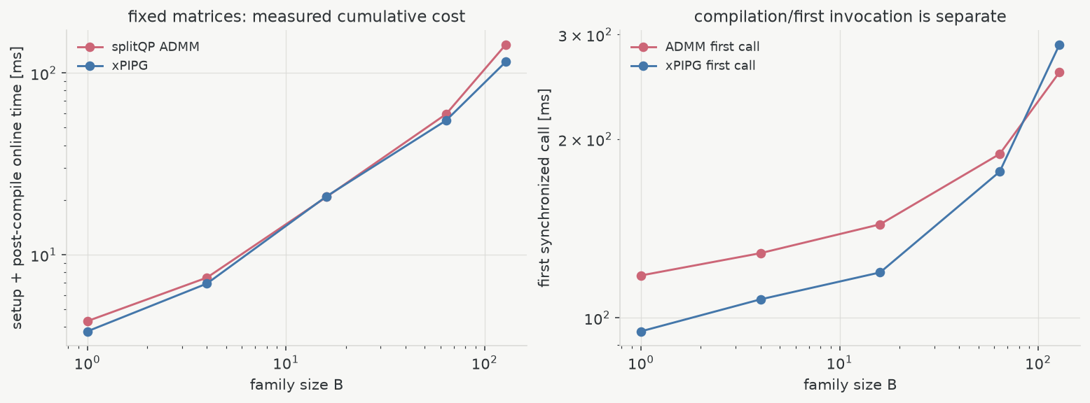
Iteration count alone is therefore an incomplete cost model. ADMM performs triangular solves and stores a factor whose fill-in depends on the matrix ordering. PIPG performs more exposed matrix–vector products and stores only vector states beyond the operators, but may need more iterations.

Computational regimes

For a small dense QP with fixed $P$ and $A$, many nearby right-hand sides, and a factorization that fits comfortably in memory, reusable-factor ADMM is a natural choice. Its implicit primal step absorbs curvature and coupling into a well-tested linear algebra kernel, and higher accuracy can justify the work spent on that kernel.

xPIPG becomes more plausible when matrices change frequently, when $P$ and $H$ are available only as matrix-free operators, or when a large independent batch maps well to accelerators. These advantages require $D$ and $K^\circ$ to have cheap projections. If either projection is a QP, or if whitening rotates a box into a difficult set, the explicit iteration has lost the property on which the comparison depends.

Poor coordinates can make either method look ineffective. ADMM then struggles with an unbalanced penalty metric or linear system; PIPG struggles with a small stable global step and weak progress in slow directions. Preconditioning must be evaluated together with presolve cost, sparsity, projection preservation, and the number of solves over which it can be amortized.

The common structure is now visible without collapsing the algorithms into one another. ADMM, PIPG, and PDHG are primal–dual fixed-point methods in which constraint residuals update a dual-like state and a transpose operator returns constraint information to primal space. ADMM realizes its main primal update through a proximal minimization; PIPGeq and PIPG use a forward gradient and explicit PI prediction–correction. In that correction, the proportional term is the current penalty gradient and the integral term is multiplier memory. xPIPG relaxes the resulting fixed-point map and makes its displacement directions observable. Which construction is preferable is a property of the problem representation and computational regime, not of the method name alone.

The executable JAX notebook implements each displayed update directly and reproduces the figures. It uses the existing splitQP ADMM implementation as the comparison and CVXPY with Clarabel only as an independent numerical reference.

References

1. Stephen Boyd, Neal Parikh, Eric Chu, Borja Peleato, and Jonathan Eckstein. Distributed Optimization and Statistical Learning via the Alternating Direction Method of Multipliers. Foundations and Trends in Machine Learning, 3(1):1–122, 2011. paper
2. Bartolomeo Stellato, Goran Banjac, Paul Goulart, Alberto Bemporad, and Stephen Boyd. OSQP: An Operator Splitting Solver for Quadratic Programs. Mathematical Programming Computation, 12:637–672, 2020. paper
3. Yue Yu, Purnanand Elango, and Behçet Açıkmeşe. Proportional-Integral Projected Gradient Method for Model Predictive Control. arXiv:2009.06980, 2020. paper
4. Yue Yu, Purnanand Elango, Ufuk Topcu, and Behçet Açıkmeşe. Proportional-Integral Projected Gradient Method for Conic Optimization. arXiv:2108.10260, 2021. paper
5. Yue Yu and Ufuk Topcu. Proportional-Integral Projected Gradient Method for Infeasibility Detection in Conic Optimization. arXiv:2109.02756, 2021. paper
6. Yue Yu, Purnanand Elango, Behçet Açıkmeşe, and Ufuk Topcu. Extrapolated Proportional-Integral Projected Gradient Method for Conic Optimization. arXiv:2203.04188, 2022. paper
7. Govind M. Chari, Yue Yu, and Behçet Açıkmeşe. Constraint Preconditioning and Parameter Selection for a First-Order Primal-Dual Method Applied to Model Predictive Control. arXiv:2403.15656, 2024. paper
8. Abhinav G. Kamath, Purnanand Elango, and Behçet Açıkmeşe. Optimal Preconditioning for Online Quadratic Cone Programming. arXiv:2501.14191, 2025. paper

The algorithmic implementations were checked against pipg-demo, optimal-preconditioning, trajopt-util, and the secondary application-specific PIPG-Cpp implementation.